3 Running Simulations

The secret of building a successful Monte Carlo simulation is to write several custom functions that work efficiently and more importantly – correctly. Then, we can:
- combine the custom functions within a single function and run the simulations using this function with nested loops, or
- write several nested loops that run each custom function independently and carry its output to the next function.
As we put the simulation functions together, we should be aware of potential errors that could either produce incorrect results or interrupt the execution of the simulation at different stages. Therefore, it is important to check all the functions carefully and patiently before running the simulations. Adding either notifications or diagnostic messages into the functions is also quite helpful for debugging problems that might occur in the functions.
Once all the simulation functions are checked, the next step is determine how to run the simulations as efficiently as possible. Loops are particularly slow in R when it comes to handling heavy computations and data operations. The apply() function collection including apply(), sapply(), and lapply() can help users avoid the loops and perform many computations and data operations very efficiently in R. For users who want to run their simulations with loops, parallel computing in R is also an excellent way to make the simulations faster. Regardless of which of these methods has been selected, it is useful to check running time of R codes – which is also known as benchmarking. We will discuss all of these steps in the remainder of Part 3.
3.1 Custom Functions
Writing custom functions does not mean that we must write every single algorithm from scratch. Instead, it means that we bring several functions (either new or existing) together so that they run the analysis that we want and return the results in the way we prefer. Going back to the hypothetical simulation scenario that we introducted in Part 1, the researcher needs several custom functions for:
- Generating response data
- Estimating item parameters
- Calculating bias, RMSE, and correlation
In the first function, we want the function to generate item parameters based on the parameter distributions that we have mentioned in Part 2 and to use these parameters to generate dichotomous response data following the 3PL model. We call this function generate_data. Our function has several arguments based on the simulation factors: nitem for the number of items, nexaminee for the number of examinees, and seed that allows us to control the random number generation. Setting the seed is very important in Monte Carlo simulations because it enables the reproducibility of simulation results. When we run the same function using the same seeds in the future, we should be able to generate the same parameters and response data.
To generate responses, we will use the sim function from the irtoys package (Partchev and Maris 2017). We could make irtoys a required package for our custom function, using require("irtoys"). This would activate the package every time we use generate_data. However, some packages can mask functions from other packages with the same names, when they are activated together within the same R session. Therefore, it is better to call the exact function that we want to use, instead of activating the entire package. Here we use irtoys::sim to call the sim function from irtoys.
Note that the three arguments, nitem, nexaminee, and seed, in the generate_data function are required. That is, all of these arguments must be specified as we run the simulations. This might create some problems in the simulation. We will talk about this in the debugging section later on.
generate_data <- function(nitem, nexaminee, seed) {
  # Set the seed
  set.seed(seed)

  # Generate item parameters
  itempar <- cbind(
    rnorm(nitem, mean = 1.13, sd = 0.25)*1.702, #a
    rnorm(nitem, mean = 0.21, sd = 0.51)*1.702, #b
    rnorm(nitem, mean = 0.16, sd = 0.05))       #c

  # Generate ability parameters
  ability <- rnorm(nexaminee, mean = 0, sd = 1)

  # Generate response data according to the 3PL model
  respdata <- irtoys::sim(ip = itempar, x = ability)
  colnames(respdata) <- paste0("item", 1:nitem)

  # Combine the generated values in a list
  data <- list(itempar = itempar,
               ability = ability,
               seed = seed,
               respdata = respdata)

  # Return the simulated data
  return(data)
}
Our function saves the item parameters, ability parameters, simulated responses, and the seed for the set.seed argument. Let’s see if our function returns what we asked for.
temp1a <- generate_data(nitem = 10, nexaminee = 1000, seed = 666)
head(temp1a$itempar)
head(temp1a$ability)
head(temp1a$respdata)
[,1] [,2] [,3]
[1,] 2.244 2.2237 0.12540
[2,] 2.780 -1.1792 0.10085
[3,] 1.772 1.1080 0.22344
[4,] 2.786 -1.1357 0.14437
[5,] 0.980 0.4738 0.16153
[6,] 2.246 0.2916 0.08589[1] 0.7550 -0.6415 1.4311 -0.6246 0.2290 0.2632 item1 item2 item3 item4 item5 item6 item7 item8 item9 item10
[1,] 0 1 1 1 1 1 1 0 1 1
[2,] 0 1 1 1 1 0 0 0 0 0
[3,] 0 1 1 1 1 1 1 0 1 1
[4,] 0 1 0 0 0 0 0 0 1 0
[5,] 0 1 1 1 1 1 1 0 1 0
[6,] 0 1 1 1 0 1 0 1 0 1Our second function is the mirt function from the mirt package (Chalmers 2019). We will create a custom function to be able to add a fixed guessing parameter and to extract the estimated item parameters. Here we will set guess as a negative value (e.g., -1), indicating that we want guessing to be freely estimated. However, if guess is greater than or equal to zero, then the guessing parameter will be fixed to this value in the function.
estimate_par <- function(data, guess = -1) {
  # If guessing is fixed
  if(guess >= 0) {

    # Model set up
    mod3PL <- mirt::mirt(data, # response data
                         1,    # unidimensional model
                         guess = guess, # fixed guessing
                         verbose = FALSE, # Don't print verbose
                         # Increase the number of EM cycles
                         # Turn off estimation messages
                         technical = list(NCYCLES = 1000,
                                          message = FALSE))
  } else {
    mod3PL <- mirt::mirt(data, # response data
                         1,    # unidimensional model
                         itemtype = "3PL", # IRT model
                         verbose = FALSE, # Don't print verbose
                         # Increase the number of EM cycles
                         # Turn off estimation messages
                         technical = list(NCYCLES = 1000,
                                          message = FALSE))
  }

  # Extract item parameters in typical IRT metric
  itempar_est <- as.data.frame(mirt::coef(mod3PL, IRTpars = TRUE, simplify = TRUE)$item[,1:3])
  return(itempar_est)
}
Let’s see if our estimate_par function can return what we want.
          a       b        g
item1 4.257  2.1529 0.123380
item2 3.192 -1.2152 0.002664
item3 1.738  1.1514 0.194192
item4 2.628 -1.1979 0.006361
item5 1.312  0.7376 0.315269
item6 2.103  0.3627 0.080536
The last function necessary for this simulation study is a summary function that will provide bias, RMSE, and correlation values for the estimated parameters. We can come up with so many solutions for this step of the simulation. We can determine the best solution based on the answers to the following questions:
Do we want to save all the simulation results and summarize them all together once all the replications are completed? This is a very safe option although saving all the results might take a lot of space or memory in the computer
Do we want to compute each evaluation index one by one and combine them in a data frame at the end? This is a good option although this would require implementing separate functions for bias, RMSE, and correlation
Can we write a single function that computes all three indices and returns them in a single data frame? This sounds more feasible because all the indices are computed together and then stored for each replication, though it might be harder to debug if a problem occurs
We wil follow the third option and create a single summary function. Note that this will return the average bias and RMSE across all items in a single replication. Therefore, we would still have to summarize the results across all replications once the simulations are complete. We create summarize as a new function which takes two arguments: est_params as the estimated parameters and true_params as the true parameters. The function will calculate bias, RMSE, and correlations among the estimated and true parameters. Then, it will return them in a long-format data set (i.e., one row per parameter and the columns indicating our evaluation indices). Not to repeat the same computations for each column (i.e., parameter), we use sapply to apply the functions so that bias, RMSE, and correlation can be calculated for the a, b, and c parameters together.
summarize <- function(est_params, true_params) {
  result <- data.frame(
    parameter = c("a", "b", "c"),
    bias = sapply(1L:3L, function(i) mean((est_params[, i] - true_params[,i]))),
    rmse = sapply(1L:3L, function(i) sqrt(mean((est_params[, i] - true_params[,i])^2))),
    correlation = sapply(1L:3L, function(i) cor(est_params[, i], true_params[,i])))
  return(result)
}
Finally, let’s test whether our final function, summarize, works properly.
  parameter       bias    rmse correlation
1         a  0.2462034 0.67355      0.7435
2         b  0.0604238 0.11273      0.9957
3         c -0.0004633 0.07805      0.4464
3.2 Debugging the Code
Debugging R codes is a rather tedious task, though this step is essential for the success of Monte Carlo simulation studies. It is important to test each custom function in a Monte Carlo simulation study as much as possible before we run them together within a single function or a loop. Otherwise, it might be harder to locate where the error occurs once the simulation begins. Especially with complex simulations, some errors might appear many hours (or even days) after we start running the simulations. Therefore, it is better to test each function in the simulation independently and then all together by following the sequence that all the functions would normally follow in the complete simulation.
In the following example, we will test one of the custom functions (generate_data) that we have created earlier. The function requires nitem, nexaminee, and seed as its arguments. What if we forget to include a seed when we are running this particular function? What would the function return? Using this example, we will review some of the debugging methods in R.
3.2.1 Custom Messages
There are many ways to find where the error occurs in R codes. An old-fashioned and yet effective way for debugging R codes is to place custom messages (similar to annotations or comments in the code) throughout the functions. If the simulation stops at a certain point in the function, we can see the latest message printed and try to find the location of the problem accordingly.
Now let’s run the generate_data function without a seed and see what happens.
Error in set.seed(seed): argument "seed" is missing, with no defaultThe output shows that the error is happening because we did not specify the seed. To fix the problem, we will revise our function by adding a condition: if seed is missing (i.e., NULL), then the function will randomly select an integer between 1 and 10,000 and use this random integer as the seed. In addition, we will add a few custom messages in the code, using cat and print. These will print messages in different forms as R runs each line of the code.
generate_data <- function(nitem, nexaminee, seed = NULL) {

  if(!is.null(seed)) {
    set.seed(seed)}
  else {
    seed <- sample.int(10000, 1)
    set.seed(seed)
    cat("Random seed = ", seed, "\n")
  }

  print("Generated item parameters")
  itempar <- cbind(
    rnorm(nitem, mean = 1.13, sd = 0.25), #a
    rnorm(nitem, mean = 0.21, sd = 0.51), #b
    rnorm(nitem, mean = 0.16, sd = 0.05)) #c

  print("Generated ability parameters")
  ability <- rnorm(nexaminee, mean = 0, sd = 1)

  print("Generated response data")
  respdata <- irtoys::sim(ip = itempar, x = ability)
  colnames(respdata) <- paste0("item", 1:nitem)

  print("Combined everything in a list")
  data <- list(itempar = itempar,
               ability = ability,
               seed = seed,
               respdata = respdata)

  # Return the simulated data
  return(data)
}
Now let’s see what our updated function would return if we forget to provide a seed.
Random seed =  7680
[1] "Generated item parameters"
[1] "Generated ability parameters"
[1] "Generated response data"
[1] "Combined everything in a list"
3.2.2 Messages and Warnings
There are other ways to add debugging-related messages into functions, such as:
message: A custom, diagnostic message created by themessage()function. The message gets printed only if a particular condition is or is not met. This does not stop the execution of the function.warning: A custom, warning message viawarning(). The message indicates that something is wrong with the function but the execution of the function continues.
Using the previous example, we will modify our function by adding a warning message showing there is no seed specified in the function and a message indicating the random seed assigned by the function itself (instead of a user-defined seed).
generate_data <- function(nitem, nexaminee, seed = NULL) {

  if(!is.null(seed)) {
    set.seed(seed)}
  else {
    warning("No seed provided!", call. = FALSE)
    seed <- sample.int(10000, 1)
    set.seed(seed)
    message("Random seed = ", seed, "\n")
  }

  itempar <- cbind(
    rnorm(nitem, mean = 1.13, sd = 0.25), #a
    rnorm(nitem, mean = 0.21, sd = 0.51), #b
    rnorm(nitem, mean = 0.16, sd = 0.05)) #c

  ability <- rnorm(nexaminee, mean = 0, sd = 1)

  respdata <- irtoys::sim(ip = itempar, x = ability)
  colnames(respdata) <- paste0("item", 1:nitem)

  data <- list(itempar = itempar,
               ability = ability,
               seed = seed,
               respdata = respdata)

  return(data)
}
What if we want to catch all errors and warnings as the function runs and store these messages to be review at the end? The answer comes from a solution offered in the R-help mailing list (see demo(error.catching):
tryCatch.W.E <- function(expr) {
  W <- NULL
  w.handler <- function(w){ # warning handler
    W <<- w
    invokeRestart("muffleWarning")
    }
  list(value = withCallingHandlers(tryCatch(expr, error = function(e) e),
                                   warning = w.handler), warning = W)
}

temp3 <- tryCatch.W.E(generate_data(nitem = 10, nexaminee = 1000))
temp3 stores both the results of generate_data and the warning message.
List of 2
 $ value  :List of 4
  ..$ itempar : num [1:10, 1:3] 1.36 1.02 1.2 1.3 1.26 ...
  ..$ ability : num [1:1000] -0.7446 0.0013 -0.8943 -0.6846 -0.8861 ...
  ..$ seed    : int 6984
  ..$ respdata: num [1:1000, 1:10] 0 1 0 0 1 1 1 0 1 1 ...
  .. ..- attr(*, "dimnames")=List of 2
  .. .. ..$ : NULL
  .. .. ..$ : chr [1:10] "item1" "item2" "item3" "item4" ...
 $ warning:List of 2
  ..$ message: chr "No seed provided!"
  ..$ call   : NULL
  ..- attr(*, "class")= chr [1:3] "simpleWarning" "warning" "condition"
Let’s see if our function returned any warnings:
<simpleWarning: No seed provided!>3.2.3 Debugging with browser()
A relatively more sophisticated way to diagnose a problem in R codes is to use browser(). This stops the execution of our codes and opens an interactive debugging screen. Using this debugging screen, we can do several things such as viewing what objects we have in the current R environment, modifying these objects, and them continuing running the code after these changes.
Now assume that users of our generate_data function must use their own seed, instead of having the function to generate one automatically. Therefore, we want to the function to stop if that occurs. We will use the stop function for this process. This function can be placed within an if statement to prevent the function for continuing – if a particular condition (or multiple conditions) occurs. Another version of this function is stopifnot which stops the function if a particular condition does not occur. To see how stopifnot works, you can type ?stopifnot in the R console and check out its help page. In the following example, we will use stop.
generate_data <- function(nitem, nexaminee, seed = NULL) {

  if(is.null(seed)) {
    stop("A seed must be provided!")}
  else {
    set.seed(seed)
  }

  print("Generated item parameters")
  itempar <- cbind(
    rnorm(nitem, mean = 1.13, sd = 0.25), #a
    rnorm(nitem, mean = 0.21, sd = 0.51), #b
    rnorm(nitem, mean = 0.16, sd = 0.05)) #c

  print("Generated ability parameters")
  ability <- rnorm(nexaminee, mean = 0, sd = 1)

  print("Generated response data")
  respdata <- irtoys::sim(ip = itempar, x = ability)
  colnames(respdata) <- paste0("item", 1:nitem)

  print("Combined everything in a list")
  data <- list(itempar = itempar,
               ability = ability,
               seed = seed,
               respdata = respdata)

  # Return the simulated data
  return(data)
}

temp3 <- generate_data(nitem = 10, nexaminee = 1000)
Running the above code above would activate the debugging mode in RStudio and the console would like this:
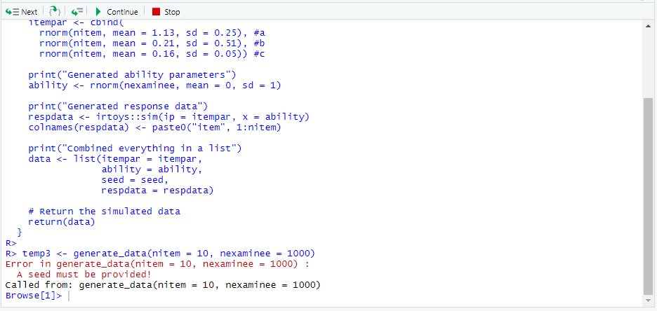
Console once the interactive debugging begins
RStudio enables the browsing mode automatically in most cases – this is why we have seen Browse[1]> after the error occured in the code. Using the browser buttons, we can evaluate the next statement, evaluate the next statement but step into the current function, execute the remainder of the function, continue executing the code until the next error or breaking point, or exit the debug mode, based on the buttons from left to right (see the figure below).

Debugging menu options
In addition to the console, the source (where we are writing the codes) would show:
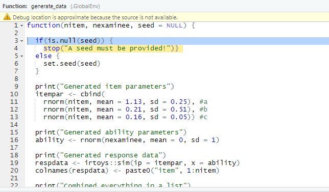
Error location in the interactive debugging
The figure above shows that the browser was able to find the location of the error. We can also activate the debugging mode for a particular function using debug(). For example, using debug(generate_data) and running temp3 <- generate_data(nitem = 10, nexaminee = 1000) will show the following output in the console. By clicking on the “next” button, we can debug the code slowly and see where the error occurred. Once we are satisfied with the function, we can turn off the interactive debugging mode using the undebug() function.
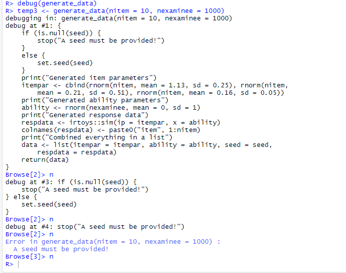
Using the debug() function
If we want to see how we came to this particular error in the function, we can hit “enter” to exit the browser mode and type traceback(). This would return the steps that we have taken until the error message:
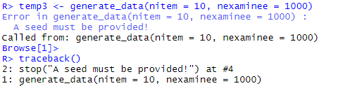
The traceback() option in R
For more further information about debugging in R, I highly recommend you to check out:
- the Debugging chapter in Hadley Wickham’s Advanced R, and
- the Debugging R Code chapter in Jennifer Bryan and Jim Hester’s What They Forgot to Teach You About R
3.3 Putting the Functions Together
As we put all the custom functions together, we must determine:
- whether we want to run each custom function separately or in a single wrapper function that simply calls all of our custom functions
- how we want to replicate our custom functions:
- the
replicatefunction - the
applyfunction collection - loops (with single cluster or parallel computing)
3.3.1 Avoding Loops
One of the easiest ways to repeat the same function without a loop is to use the replicate function in R. The way this function works is very simple. Let’s take a look at its basic structure:
Using the repeat function, we can run the generate_data function many times very quickly. For example, let’s create 5 data sets (i.e., 5 replications):
         [,1]          [,2]          [,3]          [,4]          [,5]
itempar  Numeric,30    Numeric,30    Numeric,30    Numeric,30    Numeric,30
ability  Numeric,1000  Numeric,1000  Numeric,1000  Numeric,1000  Numeric,1000
seed     8022          3891          7049          811           6957
respdata Numeric,10000 Numeric,10000 Numeric,10000 Numeric,10000 Numeric,10000
This would return an array (i.e., vector) called x which would store our simulated data sets returned from generate_data. To call a particular data set from this array (e.g., data set 1), we would use:
which would return all the components (i.e., item parameters, ability parameters, seed, and response data) from data set 1.
Another effective method to repeat a function several times without a loop is to use the apply function collection: apply(), sapply(), and lapply(). The purpose of these functions is primarily to avoid explicit uses of loops when repeating a particular task in R2. Among these three functions, sapply() and lapply() are particularly useful in simulations because they can apply an existing function (e..g, mean, median, sd) or a custom function to each element of an object. The difference between lapply() and sapply() lies between the output they return. lapply() applies a function and returns a list as its output, whereas sapply() returns a vector as its output.
In the following example, we want to extract the true item parameters from each replication stored in x. This is the first element of the output returned from generate_data. Therefore, we will use both lapply and sapply to select the first element of 5 replications stored in x.
[[1]]
[[1]]$itempar
        [,1]    [,2]    [,3]
 [1,] 1.1415 -0.3682 0.07736
 [2,] 1.3827  0.3420 0.24551
 [3,] 1.0107  0.4589 0.14046
 [4,] 0.9634  0.1928 0.10050
 [5,] 1.0133  0.7065 0.23558
 [6,] 0.9482  0.1607 0.16483
 [7,] 0.8283 -0.3466 0.11231
 [8,] 1.3640  0.3054 0.17842
 [9,] 0.5806  0.3969 0.16591
[10,] 1.8895  0.1825 0.12764


[[2]]
[[2]]$itempar
        [,1]      [,2]    [,3]
 [1,] 0.8686  0.211830 0.23417
 [2,] 1.0666 -0.647674 0.22204
 [3,] 1.3665 -0.179088 0.15410
 [4,] 0.8196  0.206515 0.19359
 [5,] 1.2334  0.005374 0.25132
 [6,] 1.0186 -0.120199 0.27701
 [7,] 1.0917 -0.096444 0.20174
 [8,] 1.1214  0.387298 0.06626
 [9,] 1.4620 -0.353471 0.18427
[10,] 0.9542 -0.386885 0.11406


[[3]]
[[3]]$itempar
        [,1]      [,2]    [,3]
 [1,] 0.8242  0.596302 0.07725
 [2,] 1.6065 -0.290621 0.17878
 [3,] 1.2838  0.728311 0.20805
 [4,] 1.0859 -0.440566 0.16173
 [5,] 1.1749 -0.045554 0.23987
 [6,] 1.1786  0.006729 0.22537
 [7,] 0.8680  1.019832 0.15020
 [8,] 1.4489 -0.435660 0.14789
 [9,] 1.4630  1.346885 0.12883
[10,] 0.5805 -0.130311 0.26612


[[4]]
[[4]]$itempar
        [,1]     [,2]    [,3]
 [1,] 1.0833 -0.62881 0.18135
 [2,] 1.4569  0.35718 0.16981
 [3,] 1.4572  0.58300 0.15132
 [4,] 0.8332  0.77767 0.19911
 [5,] 0.7998  0.84951 0.07186
 [6,] 1.2964  1.40714 0.19965
 [7,] 1.0498  0.25638 0.23851
 [8,] 1.1080 -0.58124 0.16927
 [9,] 0.7451  0.08085 0.18025
[10,] 0.8302  0.61757 0.18997


[[5]]
[[5]]$itempar
        [,1]     [,2]    [,3]
 [1,] 1.2428  0.38038 0.15683
 [2,] 0.9222  0.06897 0.14285
 [3,] 1.2159 -0.53983 0.08549
 [4,] 1.3092  0.47354 0.17746
 [5,] 1.0709 -0.15980 0.20135
 [6,] 0.8401  0.70899 0.20493
 [7,] 1.0457 -0.57915 0.19977
 [8,] 1.0311  0.96456 0.22195
 [9,] 1.4022 -0.48486 0.16690
[10,] 0.8243 -0.12529 0.11996$itempar
[,1] [,2] [,3]
[1,] 1.1415 -0.3682 0.07736
[2,] 1.3827 0.3420 0.24551
[3,] 1.0107 0.4589 0.14046
[4,] 0.9634 0.1928 0.10050
[5,] 1.0133 0.7065 0.23558
[6,] 0.9482 0.1607 0.16483
[7,] 0.8283 -0.3466 0.11231
[8,] 1.3640 0.3054 0.17842
[9,] 0.5806 0.3969 0.16591
[10,] 1.8895 0.1825 0.12764
$itempar
[,1] [,2] [,3]
[1,] 0.8686 0.211830 0.23417
[2,] 1.0666 -0.647674 0.22204
[3,] 1.3665 -0.179088 0.15410
[4,] 0.8196 0.206515 0.19359
[5,] 1.2334 0.005374 0.25132
[6,] 1.0186 -0.120199 0.27701
[7,] 1.0917 -0.096444 0.20174
[8,] 1.1214 0.387298 0.06626
[9,] 1.4620 -0.353471 0.18427
[10,] 0.9542 -0.386885 0.11406
$itempar
[,1] [,2] [,3]
[1,] 0.8242 0.596302 0.07725
[2,] 1.6065 -0.290621 0.17878
[3,] 1.2838 0.728311 0.20805
[4,] 1.0859 -0.440566 0.16173
[5,] 1.1749 -0.045554 0.23987
[6,] 1.1786 0.006729 0.22537
[7,] 0.8680 1.019832 0.15020
[8,] 1.4489 -0.435660 0.14789
[9,] 1.4630 1.346885 0.12883
[10,] 0.5805 -0.130311 0.26612
$itempar
[,1] [,2] [,3]
[1,] 1.0833 -0.62881 0.18135
[2,] 1.4569 0.35718 0.16981
[3,] 1.4572 0.58300 0.15132
[4,] 0.8332 0.77767 0.19911
[5,] 0.7998 0.84951 0.07186
[6,] 1.2964 1.40714 0.19965
[7,] 1.0498 0.25638 0.23851
[8,] 1.1080 -0.58124 0.16927
[9,] 0.7451 0.08085 0.18025
[10,] 0.8302 0.61757 0.18997
$itempar
[,1] [,2] [,3]
[1,] 1.2428 0.38038 0.15683
[2,] 0.9222 0.06897 0.14285
[3,] 1.2159 -0.53983 0.08549
[4,] 1.3092 0.47354 0.17746
[5,] 1.0709 -0.15980 0.20135
[6,] 0.8401 0.70899 0.20493
[7,] 1.0457 -0.57915 0.19977
[8,] 1.0311 0.96456 0.22195
[9,] 1.4022 -0.48486 0.16690
[10,] 0.8243 -0.12529 0.11996This is a very simple example of how lapply and sapply work. Using the same structure, we could also estimate the item parameters with mirt and save all the results together.
data <- lapply(1L:nreps,
               function(i) x[,i][4]) # the 4th part is respdata

models <- lapply(lapply(data, '[[', 'respdata'), # select respdata from each list
                 function(i) mirt::mirt(data = i, 1, itemtype = "3PL")) # apply mirt to respdata

parameters <- lapply(models,
                     function(x) mirt::coef(x, IRTpars = TRUE, simplify = TRUE)$items[,1:3])
3.3.2 Loops
Loops in R are useful when:
- there is a series of functions to be executed and
- the functions return a particular object (e.g., an integer, a data frame, or a matrix) that is necessary for the subsequent functions.
There are several control statements essential for loops:
ifandelsefor testing a condition and acting on itforfor setting up and running a loop a fixed number of iterationswhilefor executing a loop while a condition is truebreakfor stopping the execution of a loopnextfor skipping an iteration of a loop
Let’s take a quick look at how each of these control statements works:
if-else statement
if(<condition1>) {
  ## do action #1
  } else if(<condition2>)  {
    ## do action #2
    } else {
      ## do action #3
      }
for statement
for(<index1> in <values of index1>) {
  for(<index2> in <values of index2>) {
    ## do an action for each index1 and index2
  }
}
while statement
break statement
for(<index> in <values of index>) {
  ## do an action for each index
  if(<condition>) {
    break # Stop the action if condition == TRUE
  }
}
next statement
for(<index> in <values of index>) {
  if(<condition>) {
    next ## Skip the action if condition == TRUE
  }
  ## do an action for each index
}
In general, loops are very useful in Monte Carlo simulations; however, they can be very slow when:
- we are dealing with heavy computations
- we apply a function to each row or column of a large data set
Therefore, compared with traditional for loops, the apply function collection is often more preferable because it can run a computation and return its results much more quickly.
3.3.3 Parallel Computing
In some computations, creating a loop might be necessary. The regular for loop statement executes all the functions using a single processor in the computer. Similarly, the apply function collection also utilizes a single processor in the computer. The use of a single processor is the default setting in R. That is, regardless of whether we are using a 64-bit version of R in a multi-core, powerful computer, R always uses only one processor by default.
For example, in a simulation study with 100 replications via for loops, a single processor would have to run each iteration one by one and return the results once all replications are completed. This may not be a problem especially if we are running a very simple simulation. However, completing a simulation study involving heavy computations for each replication, using a single processor could be very time consuming. Fortunately, there is a solution to this problem: parallel computing3.
To benefit from parallel computing when running a Monte Carlo simulation study, we will use two packages: foreach (Microsoft and Weston 2017) and doParallel (Corporation and Weston 2019b). doParallel essentially provides a mechanism
needed to execute foreach loops in parallel computing (see the vignette for the doParallel package).
There are several steps in setting up parallel computing with doParallel:
- Make clusters for parallel computing
- Register clusters with
doParallel - Run
foreachloops using parallel computing.
Now, let’s take a look at a short example. First, we will activate doParallel. Next, we will check how many processors (i.e., cores) are available in our computer. The number of processors is the maximum number that we can use when setting up parallel computing. This would use all the processors available, though it also slows down the computer significantly and prevents us from doing other tasks in the computer. If this is a concern, then we can assign fewer processors (instead of all of them) to parallel computing.
[1] 8It seems that there are 8 processors available. We want to use 4 of these processors for running parallel loops4.
In a foreach loop, there are two ways that a loop can be set up: %do% for a regular loop and %dopar% for running the same code sequentially through multiple processors. In the following example, we will use %dopar%.
Once the simulation is over, we will turn off the clusters.
In this small example, it is hard to see the impact of parallel computing. Parallel computing will show its strengths more clearly when we check the computing time (i.e., running time) of our codes. We will talk about this in the next section.
To demonstrate how to put all the simulation functions together, we will combine the custom functions and run them together within a loop. First, we will run the latest (i.e., tested) versions of our custom functions:
# Function #1
generate_data <- function(nitem, nexaminee, seed = NULL) {

  if(!is.null(seed)) {
    set.seed(seed)}
  else {
    warning("No seed provided!", call. = FALSE)
    seed <- sample.int(10000, 1)
    set.seed(seed)
    message("Random seed = ", seed, "\n")
  }

  itempar <- cbind(
    rnorm(nitem, mean = 1.13, sd = 0.25), #a
    rnorm(nitem, mean = 0.21, sd = 0.51), #b
    rnorm(nitem, mean = 0.16, sd = 0.05)) #c

  ability <- rnorm(nexaminee, mean = 0, sd = 1)

  respdata <- irtoys::sim(ip = itempar, x = ability)
  colnames(respdata) <- paste0("item", 1:nitem)

  data <- list(itempar = itempar,
               ability = ability,
               seed = seed,
               respdata = respdata)

  return(data)
}

# Function 2
estimate_par <- function(data, guess = -1) {
  # If guessing is fixed
  if(guess >= 0) {

    # Model set up
    mod3PL <- mirt::mirt(data, # response data
                         1,    # unidimensional model
                         guess = guess, # fixed guessing
                         verbose = FALSE, # Don't print verbose
                         # Increase the number of EM cycles
                         # Turn off estimation messages
                         technical = list(NCYCLES = 1000,
                                          message = FALSE))
  } else {
    mod3PL <- mirt::mirt(data, # response data
                         1,    # unidimensional model
                         itemtype = "3PL", # IRT model
                         verbose = FALSE, # Don't print verbose
                         # Increase the number of EM cycles
                         # Turn off estimation messages
                         technical = list(NCYCLES = 1000,
                                          message = FALSE))
  }

  # Extract item parameters in typical IRT metric
  itempar_est <- as.data.frame(mirt::coef(mod3PL, IRTpars = TRUE, simplify = TRUE)$item[,1:3])
  return(itempar_est)
}

# Function #3
summarize <- function(est_params, true_params) {
  result <- data.frame(
    parameter = c("a", "b", "c"),
    bias = sapply(1L:3L, function(i) mean((est_params[, i] - true_params[,i]))),
    rmse = sapply(1L:3L, function(i) sqrt(mean((est_params[, i] - true_params[,i])^2))),
    correlation = sapply(1L:3L, function(i) cor(est_params[, i], true_params[,i])))
  return(result)
}
Second, we will set up our simulation conditions so that it would be easier to update them as we run all the conditions. Note that the number of iterations (i.e., replications) is only 4 for now. If the functions work as expected, we will increase the number of iterations to 100.
iterations = 4 # Only 4 iteration for now
seed = sample.int(10000, 100)
nitem = 10 # 10, 15, 20, or 25
nexaminee = 1000 # 250, 500, 750, or 1000
guess = -1 # A negative value or a value from 0 to 1
Third, we will set up parallel computing and register multiple processors for the simulation.
Finally, we will run our simulation and save the results as simresults.
simresults <- foreach(i=1:iterations,
                      .packages = c("mirt", "doParallel"),
                      .combine = rbind) %dopar% {
                        # Generate item parameters and data
                        step1 <- generate_data(nitem=nitem, nexaminee=nexaminee, seed=seed[i])
                        # Estimate item parameters
                        step2 <- estimate_par(step1$respdata, guess = guess)
                        # Summarize results
                        summarize(step2, step1$itempar)
                        }
Now, we can see the results (assuming no error messages appeared on our console):
   parameter      bias   rmse correlation
1          a  0.128163 0.3748     0.78904
2          b -0.059314 0.5941     0.62520
3          c -0.025765 0.1377     0.24511
4          a -0.030007 0.3135     0.49103
5          b -0.244383 0.4692     0.88362
6          c -0.052045 0.1444    -0.27393
7          a  0.199876 0.7391    -0.08689
8          b  0.017008 0.2874     0.82013
9          c  0.002217 0.1187     0.13883
10         a  0.310501 0.4886     0.78836
11         b  0.129384 0.3310     0.84102
12         c  0.072968 0.1203     0.42944
Remember that this is only for one of the crossed conditions (10 items, 1000 examinees, no fixed guessing) across four iterations. We can summarize the results across all iterations, add additional information to remind us what we have done in the simulation, and save the results. We will use the dplyr package (Wickham, François, et al. 2019) for summarizing our simulation results.
library("dplyr")

simresults_final <- simresults %>%
  group_by(parameter) %>%
  # Find the average and rounded values
  summarise(bias = round(mean(bias),3),
            rmse = round(mean(rmse),3),
            correlation = round(mean(correlation),3)) %>%
  mutate(nitem = nitem,
         nexaminee = nexaminee,
         guess = guess) %>%
  select(nitem, nexaminee, guess, parameter, bias, rmse, correlation) %>%
  as.data.frame()

simresults_final
nitem nexaminee guess parameter bias rmse correlation
1 10 1000 -1 a 0.152 0.479 0.495
2 10 1000 -1 b -0.039 0.420 0.792
3 10 1000 -1 c -0.001 0.130 0.135We can also create a nested loop where we can all the conditions together. Here we use %:% to set up three nested loops without curly brackets. The final loop contains %dopar% with curly brackets and closes all the loops. Note that we included the final summary function (see how step3 is summarized) inside these nested loops. This will return a long-format summary data set with all the conditions based on 100 iterations.
# Set all the conditions
iterations = 100
seed = sample.int(10000, 100)
nitem = c(10, 15, 20, 25)
nexaminee = c(250, 500, 750, 1000)
guess = c(-1, 0.16)

# Register four clusters
cl <- makeCluster(4)
registerDoParallel(cl)

# Run nested foreach loops
simresults <- foreach(i=1:iterations,
                      .packages = c("mirt", "doParallel", "dplyr"),
                      .combine = rbind) %:%
  foreach(j=nitem,
          .packages = c("mirt", "doParallel", "dplyr"),
          .combine = rbind)  %:%

 foreach(k=nexaminee,
          .packages = c("mirt", "doParallel", "dplyr"),
          .combine = rbind)  %:%

  foreach(m=guess,
          .packages = c("mirt", "doParallel", "dplyr"),
          .combine = rbind)  %dopar% {
            # Generate item parameters and data
            step1 <- generate_data(nitem=j, nexaminee=k, seed=seed[i])
            # Estimate item parameters
            step2 <- estimate_par(step1$respdata, guess = m)
            # Summarize results
            step3 <- summarize(step2, step1$itempar)
            # Finalize results
            step3 %>%
              group_by(parameter) %>%
              summarise(bias = round(mean(bias),3),
                        rmse = round(mean(rmse),3),
                        correlation = round(mean(correlation),3)) %>%
              mutate(nitem = j,
                     nexaminee = k,
                     guess = m) %>%
              select(nitem, nexaminee, guess, parameter, bias, rmse, correlation) %>%
              as.data.frame()
          }

# Stop the clusters
stopCluster(cl)
If you are interested in high performance computing, I also recommend the following resources:
- Lim and Tjhi’s book: R High Performance Programming
- The Performance chapter in Hadley Wickham’s Advanced R book
3.4 Benchmarking
There are several options to measure running time of a Monte Carlo simulation in R.
- Functions included in base
R:
system.time()Sys.time()Rprof()andsummaryRprof()
- Packages on benchmarking
- The
tictocpackage (Izrailev 2014) - The
rbenchmarkpackage (Kusnierczyk 2012) - The
microbenchmarkpackage (Mersmann 2019) - The
benchpackage (Hester 2020) (check out its website)
The three packages, rbenchmark, microbenchmark, and bench, provide detailed information about running time as well as memory usage in R. Furthermore, microbenchmark and bench are capable of visualizing benchmarking results (utilizing ggplot2). For more information on benchmarking in R, I recommend you to check out this nice blog post.
In the following example, we will run a simple benchmarking test using our simulation. We will use %do% and %dopar% to see the difference. We will use both system.time and Sys.time together.
iterations = 4 #Eventually this will be 100
seed = sample.int(10000, 100)
nitem = 10 #10, 15, 20, or 25
nexaminee = 1000 #250, 500, 750, or 1000
guess = -1 # A negative value or a value from 0 to 1

# No parallel computing
start_time <- Sys.time() # Starting time
system.time(
  simresults <- foreach(i=1:iterations,
                        .packages = c("mirt", "doParallel"),
                        .combine = rbind) %do% {
                          # Generate item parameters and data
                          step1 <- generate_data(nitem=nitem, nexaminee=nexaminee, seed=seed[i])
                          # Estimate item parameters
                          step2 <- estimate_par(step1$respdata, guess = guess)
                          # Summarize results
                          summarize(step2, step1$itempar)
                        }
)
user system elapsed
8.34 0.09 8.50 Time difference of 8.631 secs# With parallel computing
start_time <- Sys.time() # Starting time
system.time(
simresults <- foreach(i=1:iterations,
.packages = c("mirt", "doParallel"),
.combine = rbind) %dopar% {
# Generate item parameters and data
step1 <- generate_data(nitem=nitem, nexaminee=nexaminee, seed=seed[i])
# Estimate item parameters
step2 <- estimate_par(step1$respdata, guess = guess)
# Summarize results
summarize(step2, step1$itempar)
}
) user system elapsed
0.02 0.01 3.23 Time difference of 3.384 secsIn the output returned from system.time, “elapsed” is the time taken to execute the entire process, “user” gives the CPU time spent by the current process (i.e., the current R session), and “system” gives the CPU time spent by the kernel (the operating system) on behalf of the current process (see this post on R-help mailing list for further information).
What if we want to see the time taken by each function in the whole simulation? Rprof() provides us with this type of information. To activate profiling in R, we need to run:
Then, we can see the running time of each function after profiling has been activated. We can use summaryRprof() to export the results at the end. We wil do this step for a single iteration to see the time distribution across all functions5.
Rprof() # Turn on profiling
# Generate item parameters and data
step1 <- generate_data(nitem=nitem, nexaminee=nexaminee, seed=seed[1])
# Estimate item parameters
step2 <- estimate_par(step1$respdata, guess = guess)
# Summarize results
step3 <- summarize(step2, step1$itempar)
summaryRprof()$by.self
self.time self.pct total.time total.pct
"Estep.mirt" 0.78 33.05 0.84 35.59
"computeItemtrace" 0.38 16.10 0.40 16.95
"LogLikMstep" 0.24 10.17 0.62 26.27
"gr" 0.16 6.78 0.18 7.63
"<Anonymous>" 0.10 4.24 1.12 47.46
"EM.group" 0.08 3.39 2.34 99.15
"fn" 0.06 2.54 0.80 33.90
"reloadPars" 0.06 2.54 0.12 5.08
"ifelse" 0.06 2.54 0.06 2.54
"FUN" 0.04 1.69 2.34 99.15
"getClassDef" 0.04 1.69 0.08 3.39
"getCallingDLLe" 0.04 1.69 0.06 2.54
"match.arg" 0.04 1.69 0.04 1.69
"tryCatch" 0.02 0.85 2.36 100.00
"optim" 0.02 0.85 1.06 44.92
"Estep" 0.02 0.85 0.86 36.44
"mahalanobis" 0.02 0.85 0.14 5.93
"order" 0.02 0.85 0.06 2.54
"%*%" 0.02 0.85 0.02 0.85
"%in%" 0.02 0.85 0.02 0.85
".getClassesFromCache" 0.02 0.85 0.02 0.85
"as.matrix" 0.02 0.85 0.02 0.85
"attr" 0.02 0.85 0.02 0.85
"c" 0.02 0.85 0.02 0.85
"get0" 0.02 0.85 0.02 0.85
"longpars_constrain" 0.02 0.85 0.02 0.85
"methodsPackageMetaName" 0.02 0.85 0.02 0.85In the output, “self.pct” is the most important column because it indicates the percentage of time that each of the listed tasks has taken in the estimation process.
Next, let’s see how the tictoc package works for finding running time of our code. Between each tic() and toc(), it saves the time spent. So, we place several tic() and toc() functions. The first one, tic("Total simulation time:") will be closed at the end so that we can see the total time spent on the simulation. The others in between will calculate the time for each step (i.e., step 1, step 2, and step 3).
library("tictoc")
tic("Total simulation time:")
tic("Generate item parameters and data")
step1 <- generate_data(nitem=nitem, nexaminee=nexaminee, seed=seed[1])
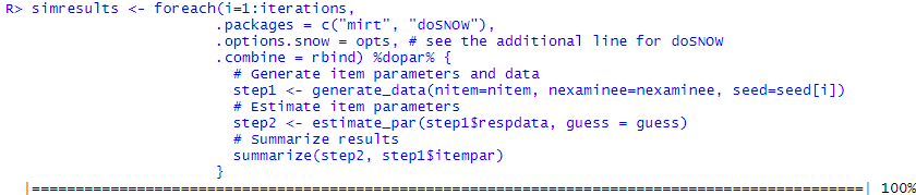
toc()Generate item parameters and data: 0 sec elapsedEstimate item parameters: 2.65 sec elapsedSummarize results: 0 sec elapsedTotal simulation time:: 2.65 sec elapsedFinally, let’s add a progress bar to our simulation study. We will use the txtProgressBar function from base R and the doSNOW package (Corporation and Weston 2019a) together. The txtProgressBar function is a standalone function and thus it does not require other packages to print a progress bar. However, in the following example, we will do parallel computing using the doSNOW package (it is very similar to doParallel) and add a progress bar into our simulation. This will require us to add .options.snow in the loop so that the progress bar works along with the simulation.
iterations = 10 #Eventually this will be 100
seed = sample.int(10000, 100)
nitem = 10 #10, 15, 20, or 25
nexaminee = 1000 #250, 500, 750, or 1000
guess = -1 #A negative value or a value from 0 to 1

library("doSNOW")
cl <- makeCluster(4)
registerDoSNOW(cl)

# Set up the progress bar
pb <- txtProgressBar(max = iterations, style = 3) # Initiate progress bar
progress <- function(n) {setTxtProgressBar(pb, n)}
opts <- list(progress = progress)

# Run the simulation
simresults <- foreach(i=1:iterations,
                      .packages = c("mirt", "doSNOW"),
                      .options.snow = opts, # see the additional line for doSNOW
                      .combine = rbind) %dopar% {
                        # Generate item parameters and data
                        step1 <- generate_data(nitem=nitem, nexaminee=nexaminee, seed=seed[i])
                        # Estimate item parameters
                        step2 <- estimate_par(step1$respdata, guess = guess)
                        # Summarize results
                        summarize(step2, step1$itempar)
                      }
close(pb) # Close progress bar
stopCluster(cl)
As the simulation progresses, we should see a progress bar with a percent sign at the end, which is style = 3 in the txtProgressBar function6. Once the simulation is complete, we should see the following screen in the console:
Status of progress bar once the simulation is complete
References
Chalmers, Phil. 2019. Mirt: Multidimensional Item Response Theory. https://CRAN.R-project.org/package=mirt.
Corporation, Microsoft, and Stephen Weston. 2019a. DoSNOW: Foreach Parallel Adaptor for the ’Snow’ Package. https://CRAN.R-project.org/package=doSNOW.
Corporation, Microsoft, and Steve Weston. 2019b. DoParallel: Foreach Parallel Adaptor for the ’Parallel’ Package. https://CRAN.R-project.org/package=doParallel.
Hester, Jim. 2020. Bench: High Precision Timing of R Expressions. https://CRAN.R-project.org/package=bench.
Izrailev, Sergei. 2014. Tictoc: Functions for Timing R Scripts, as Well as Implementations of Stack and List Structures. https://CRAN.R-project.org/package=tictoc.
Kusnierczyk, Wacek. 2012. Rbenchmark: Benchmarking Routine for R. https://CRAN.R-project.org/package=rbenchmark.
Mersmann, Olaf. 2019. Microbenchmark: Accurate Timing Functions. https://CRAN.R-project.org/package=microbenchmark.
Microsoft, and Steve Weston. 2017. Foreach: Provides Foreach Looping Construct for R. https://CRAN.R-project.org/package=foreach.
Partchev, Ivailo, and Gunter Maris. 2017. Irtoys: A Collection of Functions Related to Item Response Theory (Irt). https://CRAN.R-project.org/package=irtoys.
Wickham, Hadley, Romain François, Lionel Henry, and Kirill Müller. 2019. Dplyr: A Grammar of Data Manipulation. https://CRAN.R-project.org/package=dplyr.
See the Guru99 website for more information on these functions.↩
For a quick introduction to parallel computing in
R, you can check out this website.↩If the computer has a Mac operating system, then
cl <- makeCluster(4, outfile="")should be used.↩The results would be very similar across all iterations using the same conditions.↩
There are also styles 1 and 2. Check out
?txtProgressBarfor examples.↩