Explanatory IRT for Dichotomous Data

The following example shows how to use item-related and person-related explanatory variables to explain dichotomous responses in the verbal aggression data set.

data("VerbAgg")

mod2a <- eirm(formula = "r2 ~ -1 + situ + btype + mode + (1|id)", data = VerbAgg)

print(mod2a)

## EIRM formula: "r2 ~ -1 + situ + btype + mode + (1|id)" 
## 
## Number of persons: 316 
## 
## Number of observations: 7584 
## 
## Number of predictors: 5 
## 
## Parameter Estimates:
## 
##              Easiness       S.E.   z-value       p-value
## situother   1.7437027 0.10145090  17.18765  3.285796e-66
## situself    0.7158127 0.09775376   7.32261  2.431943e-13
## btypescold -1.0551642 0.06803581 -15.50895  3.017583e-54
## btypeshout -2.0421978 0.07292877 -28.00263 1.509082e-172
## modedo     -0.6715770 0.05621055 -11.94753  6.688613e-33
## 
## Note: The estimated parameters above represent 'easiness'.
## Use difficulty = TRUE to get difficulty parameters.

It is possible to visualize the parameters using an item-person map using plot(mod2a), which returns the following plot:

plot(mod2a)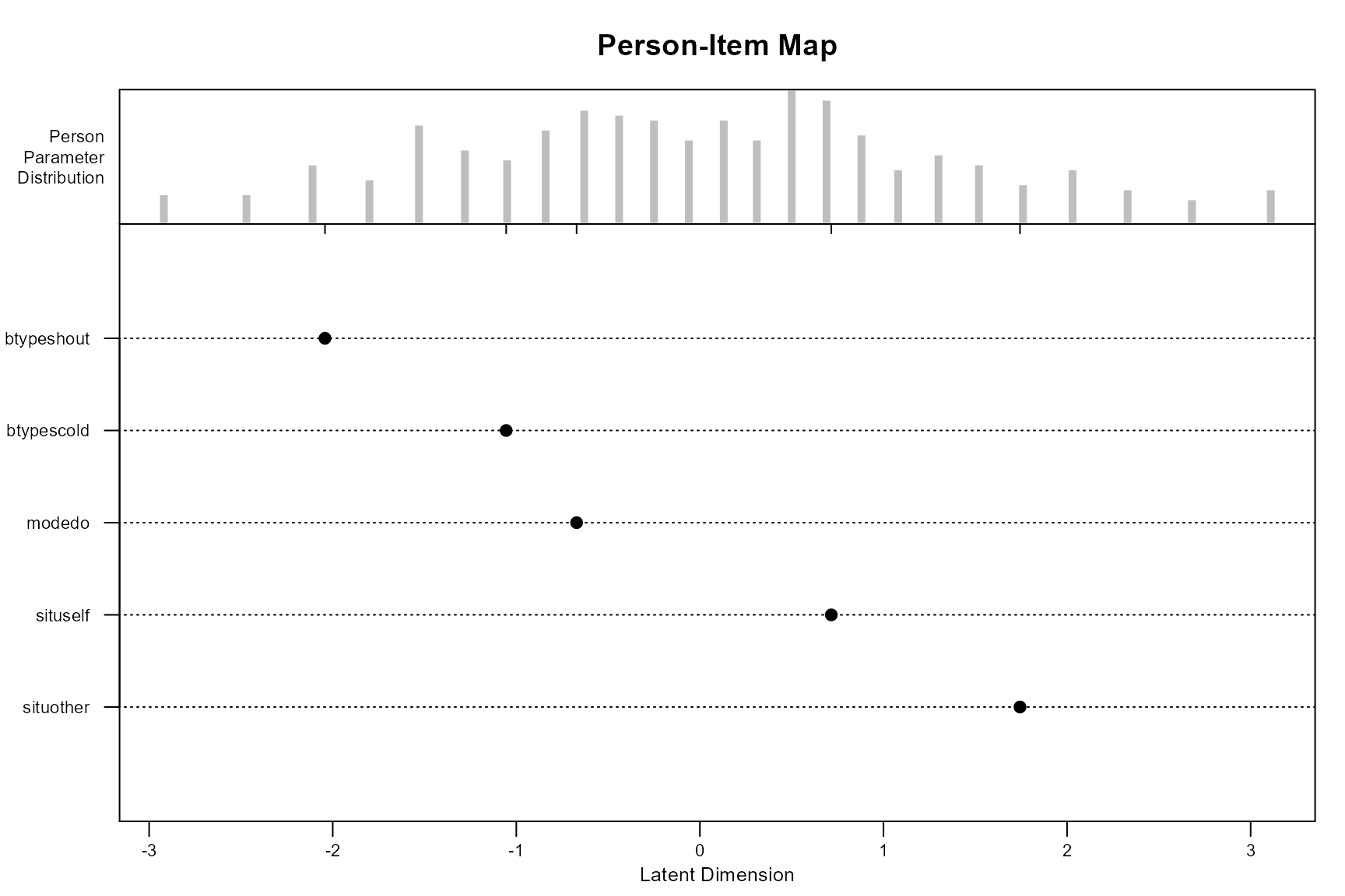

In addition to the item-person map, we can also visualize the marginal effects in the model using the marginalplot function. This plot uses the ggeffects package to calculate the marginal effects and the ggplot2 package to create a plot. The following code will return a marginal effect plot with the three explanatory variables in mod2a.

marginalplot(mod2a, predictors = c("situ", "btype", "mode"))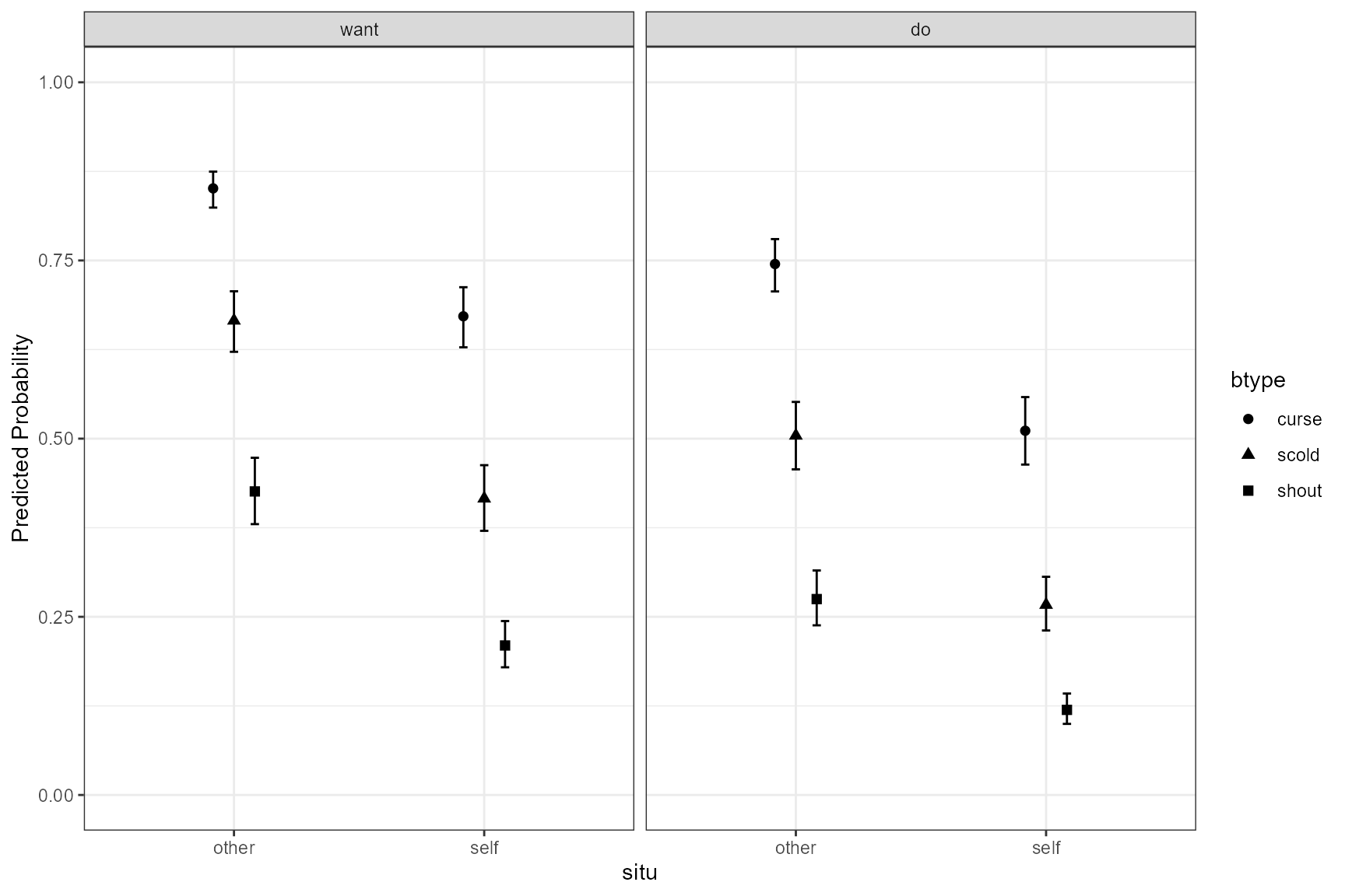

Lastly, we can compare nested explanatory models with each other. The following example shows the estimation of a more compact version of mod2a with one less variable and compares the two models (i.e., mod2a vs. mod2b).

mod2b <- eirm(formula = "r2 ~ -1 + situ + btype + (1|id)", data = VerbAgg)

anova(mod2a$model, mod2b$model)

## Data: data
## Models:
## mod2b$model: r2 ~ -1 + situ + btype + (1 | id)
## mod2a$model: r2 ~ -1 + situ + btype + mode + (1 | id)
##             npar    AIC    BIC  logLik deviance  Chisq Df Pr(>Chisq)    
## mod2b$model    5 8389.6 8424.2 -4189.8   8379.6                         
## mod2a$model    6 8249.9 8291.5 -4119.0   8237.9 141.62  1  < 2.2e-16 ***
## ---
## Signif. codes:  0 '***' 0.001 '**' 0.01 '*' 0.05 '.' 0.1 ' ' 1

Okan Bulut

2022-01-22