Introduction to R and RStudio
R and RStudio

What is R?
- is a free, open source program for statistical computing and data visualization.
- is cross-platform (e.g., available on Windows, Mac OS, and Linux).
- is maintained and regularly updated by the Comprehensive R Archive Network (CRAN).
- is capable of running all types of statistical analyses.
- has amazing visualization capabilities (high-quality, customizable figures).
- enables reproducible research.
- has many other capablities, such as web programming.
- supports user-created packages (currently, more than 10,000)
What is RStudio?
- is a free program available to control R.
- provides a more user-friendly interface for R.
- includes a set of tools to help you be more productive with R, such
as:
- A syntax-highlighting editor for highlighting your R codes
- Functions for helping you type the R codes (auto-completion)
- A variety of tools for creating and saving various plots (e.g., histograms, scatterplot)
- A workspace management tool for importing or exporting data
Setting up R and RStudio
To benefit from RStudio, both R and RStudio should be installed in your computer. R and RStudio are freely available from the following websites:
To download and install R:
- Go to https://cran.r-project.org/
- Click “Download R for Mac/Windows””
- Download the appropriate file: • Windows users click Base, and download the installer for the latest R version • Mac users select the file R-4.X.X.pkg that aligns with your OS version
- Follow the instructions of the installer.
Important: If you are using a Windows computer, you must also install Rtools.
To download and install RStudio:
- Go to https://posit.co/download/rstudio-desktop/
- Click “Download” under Step 2: Install RStudio Desktop
- Select the install file for your OS
- Follow the instructions of the installer.
After you open RStudio, you should see the following screen:
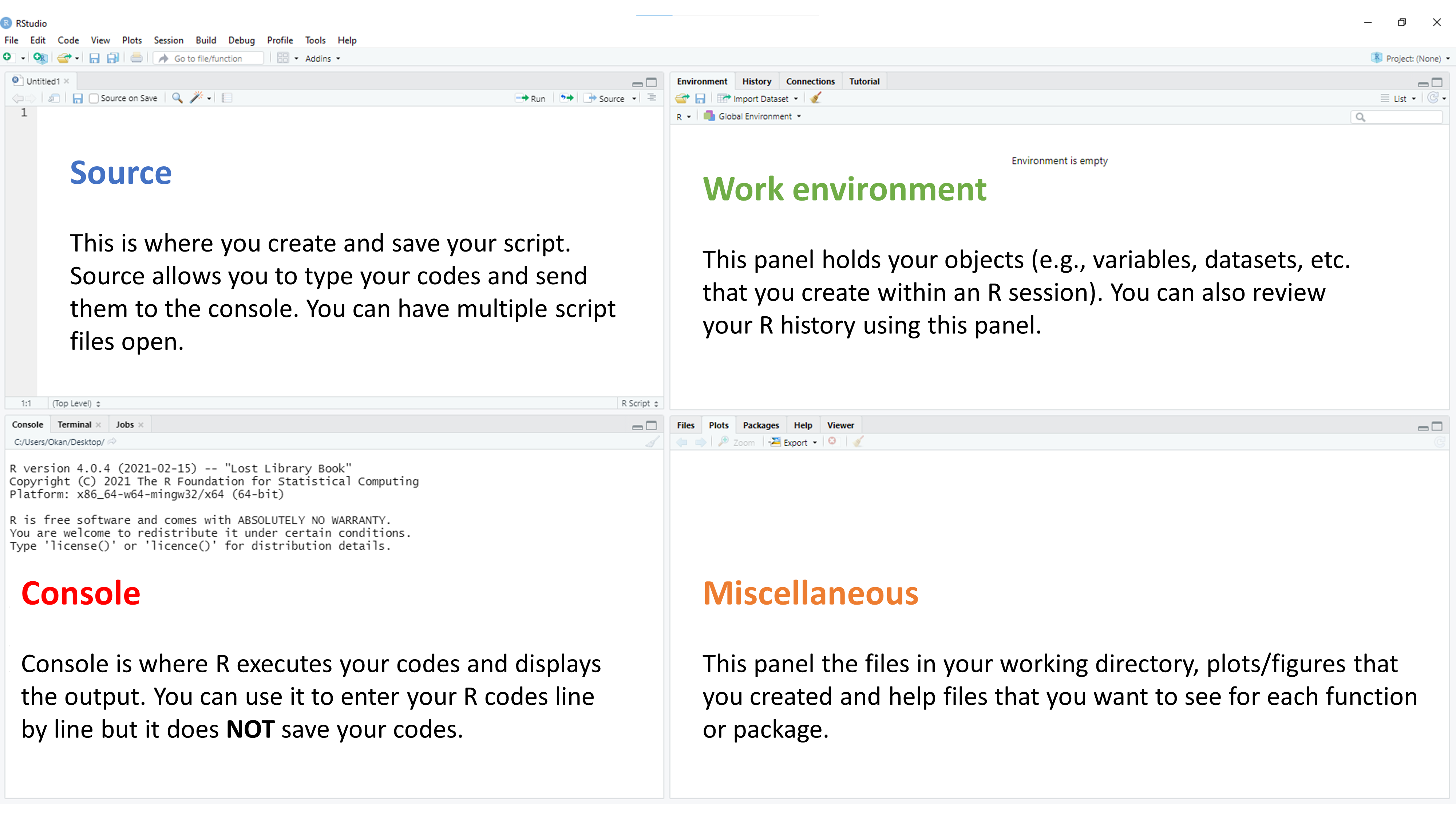
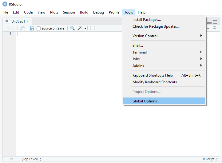
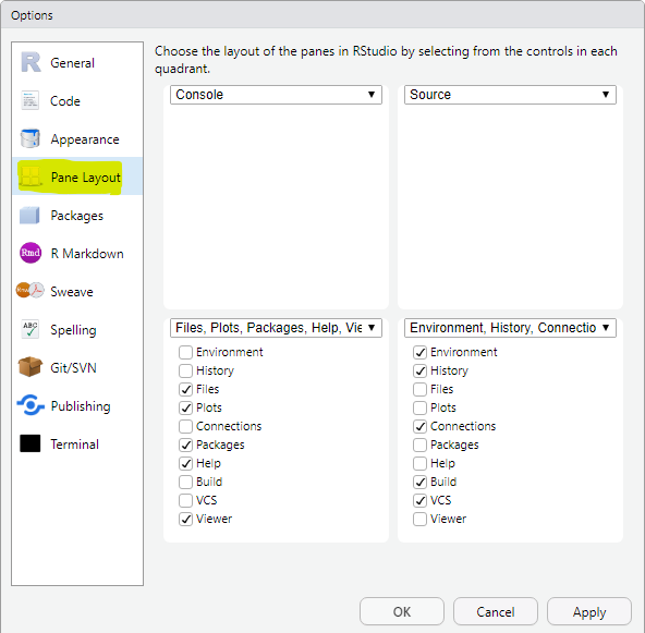
I personally prefer console on the top-left, source on the top-right, files on the bottom-left, and environment on the bottom-right. The pane layout can be updated using Global Options under Tools.
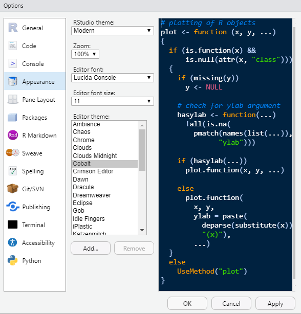
We can also change the appearance (e.g., code highlighting, font type, font size, etc.). For example, I prefer to use the Cobalt editor theme due to its dark background and contrasting colors:
Note: To get yourself more familiar with RStudio, I recommend you to check out the RStudio cheatsheet and Oscar Torres-Reyna’s nice tutorial.
Creating a new script
In R, we can type our commands in the console; but once we close R, everything we have typed will be gone. Therefore, we should create an empty script, write the codes in the script, and save it for future use. We can replicate the exact same analysis and results by running the script again later on. The R script file has the .R extension, but it is essentially a text file. Thus, any text editor (e.g., Microsoft Word, Notepad, TextPad) can be used to open a script file for editing outside of the R environment.
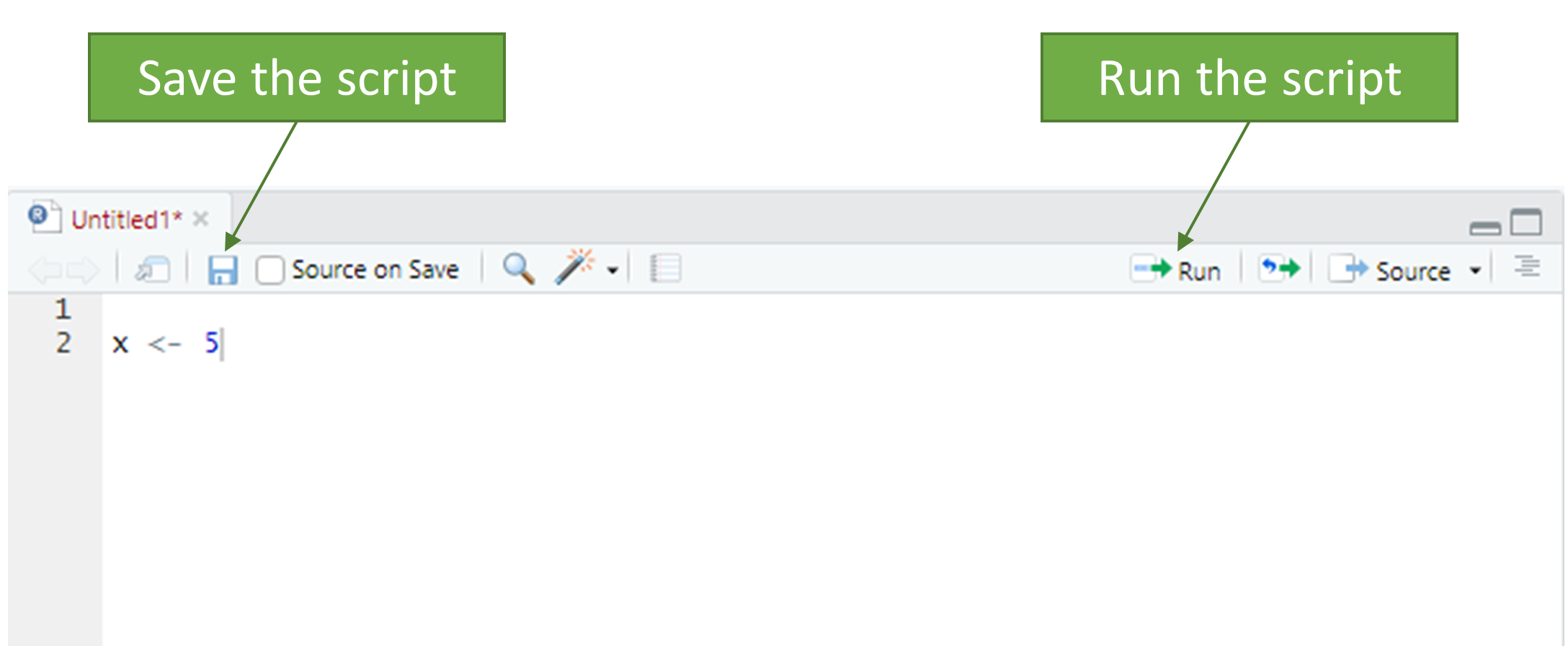
We can create a new script file in R as follows:
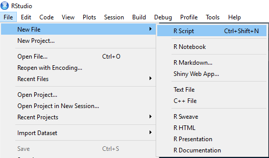
When we type some codes in the script, we can select the lines we want to run and then hit the run button. Alternatively, we can bring the cursor at the beginning of the line and hit the run button which runs one line at a time and moves to the next line.
Changing working directory
An important feature of R is “working directory”, which refers to a
location or a folder in your computer where you keep your R script, your
data files, etc. Once we define a working directory in R, any data file
or script within that directory can be easily imported into R without
specifying where the file is located. By default, R chooses a particular
location in your computer (typically Desktop or Documents) as your
working director. To see our current working director, we need to run a
getwd() command in the R console:
This will return a path like this:
Once we decide to change the current working direcory into a different location, we can do it in two ways:
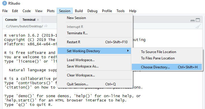
Method 1: Using the “Session” options menu in RStudio
We can select Session > Set Working Directory > Choose Directory to find a folder or location that we want to set as our current working directory.
Method 2: Using the setwd command in
the console
Tpying the following code in the console will set a hypothetical “edpy507” folder on my desktop as the working directory. If the folder path is correct, R changes the working directory without giving any error messages in the console.
To ensure that the working directory is properly set, we can use the
getwd() command again:
IMPORTANT: R does not accept any backslashes in the file path. Instead of a backslash, we need to use a frontslash. This is particulary important for Windows computers since the file paths involve backslashes (Mac OS X doesn’t have this problem).
Downloading and installing R packages
The base R program comes with many built-in functions to compute a variety of statistics and to create graphics (e.g., histograms, scatterplots, etc.). However, what makes R more powerful than other software programs is that R users can write their own functions, put them in a package, and share it with other R users via the CRAN website.
For example, ggplot2 (Wickham et
al., 2021) is a well-known R package, created by Hadley Wickham
and Winston Chang. This package allows R users to create elegant data
visualizations. To download and install the ggplot2
package, we need to use the install.packages command. Note
that your computer has to be connected to the internet to be able to
connect to the CRAN website and download the package.
Once a package is downloaded and installed, it is permanently in your
R folder. That is, there is no need to re-install it, unless you remove
the package or install a new version of R. These downloaded packages are
not directly accessible until we activate them in your R session.
Whenever we need to access a package in R, we need to use the
library command to activate it. For example, to access the
ggplot2 package, we would use:
We can use the analogy of buying books from a bookstore
(install.packages) and adding them to your personal library
(library) to remember how these two commands work.

Basics of the R language
Creating new variables
To create a new variable in R, we use the assignment operator,
<-. To create a variable x that equals 25,
we need to type:
If we want to print x, we just type x in
the console and hit enter. R returns the value assigned to
x.
[1] 25We can also create a variable that holds multiple values in it, using
the c command (c stands for
combine).
[1] 60 72 80 84 56[1] 1.70 1.75 1.80 1.90 1.60Once we create a variable, we can do further calculations with it.
Let’s say we want to transform the weight variable (in kg)
to a new variable called weight2 (in lbs).
[1] 132.2772 158.7326 176.3696 185.1881 123.4587Note that we named the variable as weight2. So, both
weight and weight2 exist in the active R
session now. If we used the following, this would overwrite the existing
weight variable.
We can also define a new variable based on existing variables.
[1] 170 140 110 82 135Sometimes we need a variable that holds character strings rather than
numerical values. If a value is not numerical, we need to use double
quotation marks. In the example below, we create a new variable called
cities that has four city names in it. Each city name is
written with double quotation marks.
[1] "Edmonton" "Calgary" "Red Deer" "Spruce Grove"We can also treat numerical values as character strings. For example,
assume that we have a gender variable where 1=Male and
2=Female. We want R to know that these values are not actual numbers;
instead, they are just numerical labels for gender groups.
[1] "1" "2" "2" "1" "2"Important rules of the R language
Here is a list of important rules for using the R language more effectively:
- Case-sensitivity: R codes written in lowercase would NOT refer to the same codes written in uppercase.
cities <- c("Edmonton", "Calgary", "Red Deer", "Spruce Grove")
Cities
CITIES

Error: object 'Cities' not found
Error: object 'CITIES' not found- Variable names: A variable name cannot begin with a number or include a space.
4cities <- c("Edmonton", "Calgary", "Red Deer", "Spruce Grove")
my cities <- c("Edmonton", "Calgary", "Red Deer", "Spruce Grove")

Error: unexpected symbol in "4cities"
Error: unexpected symbol in "my cities"- Naming conventions: I recommend using consistent
and clear naming conventions to keep the codes clear and organized. I
personally prefer all lowercase with underscore (e.g.,
my_variable). The other naming conventions are:
- All lowercase: e.g.
mycities - Period.separated: e.g.
my.cities - Underscore_separated: e.g.
my_cities - Numbers at the end: e.g.
mycities2018 - Combination of some of these rules:
my.cities.2018
- Commenting: The hashtag symbol (#) is used for commenting in R. Any words, codes, etc. coming after a hashtag are just ignored. I strongly recommend you to use comments throughout your codes. These annotations would remind you what you did in the codes and why you did it that way. You can easily comment out a line without having to remove it from your codes.
# Here I define four cities in Alberta
cities <- c("Edmonton", "Calgary", "Red Deer", "Spruce Grove")
Importing data into R
We often save our data sets in convenient data formats, such as Excel, SPSS, or text files (.txt, .csv, .dat, etc.). R is capable of importing (i.e., reading) various data formats.
There are two ways to import a data set into R:
- By using the “Import Dataset” menu option in RStudio
- By using a particular R command
Method 1: Using RStudio
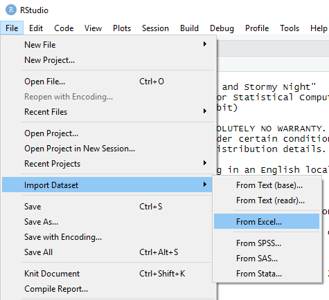
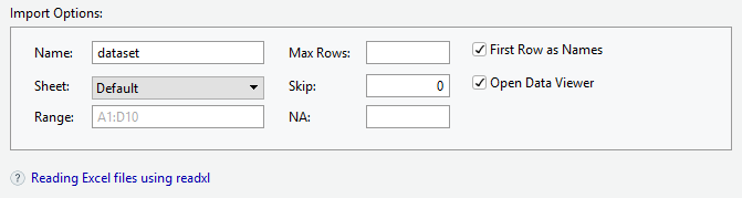
Importing Excel files
- Browse for the file that you want to import
- Give a name for the data set
- Choose the sheet to be imported
- “First Row as Names” if the variable names are in the first row of the file.
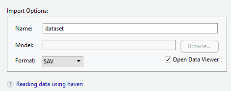
Importing SPSS files
- Browse the file that you want to import
- Give a name for the data set
- Choose the SPSS data format (SAV)
Method 2: Using R commands
R has some built-in functions, such as read.csv and
read.table. Also, there are R packages for importing
specific data formats. For example, foreign for SPSS files
and xlsx for Excel files. Here are some examples:
Importing Excel files
# Install and activate the package first
install.packages("xlsx")
library("xlsx")

# Use read.xlsx to import an Excel file
my_excel_file <- read.xlsx("path to the file/filename.xlsx", sheetName = "sheetname")
Importing SPSS files
# Install and activate the package first
install.packages("foreign")
library("foreign")

# Use read.spss to import an SPSS file
my_spss_file <- read.spss("path to the file/filename.sav", to.data.frame = TRUE)
Importing text files
# No need to install any packages
# R has many built-in functions already

# A comma-separated-values file with a .csv extension
my_csv_file <- read.csv("path to the file/filename.csv", header = TRUE)

# A tab delimited text file with .txt extension
my_txt_file <- read.table("path to the file/filename.txt", header = TRUE, sep = "\t")
Here we should note that:
header = TRUEif the variable names are in the first row; otherwise, useheader = FALSEsep="\t"for tab-separated files;sep=","for comma-separated files
Self-help
In the spirit of open-source, R is very much a self-guided tool. We can look for solutions to R-related problems in multiple ways:
- To get help on installed packages (e.g., what’s inside this package):
# To get details regarding contents of a package
help(package = "ggplot2")

# To list vignettes available for a specific package
vignette(package = "ggplot2")

# To view specific vignette
vignette("ggplot2-specs")
Use the
?to open help pages for functions or packages (e.g., try running?summaryin the console to see how thesummaryfunction works).For tricky questions and funky error messages (there are many of these), use Google (include “in R” to the end of your query).
StackOverflow (https://stackoverflow.com/) has become a great resource with many questions for many specific packages in R, and a rating system for answers.
Finally, you can simply search your question on Google! With the right keywords, you can find the answers to even very complex questions about R. Here are a few tips and tricks to help you find information on Google.