Classical Test Theory (CTT)
Example 1: The Need for Cognition Scale
Need for cognition, or shortly NFC, is a psychological latent trait defined as the desire to engage in cognitively challenging tasks and effortful thinking (Cacioppo & Petty, 1982). Individuals with high levels of NFC tend to seek, acquire, think about, and reflect on information, whereas individuals with low levels of NFC tend to avoid detailed information about the world and find cognitively complex tasks stressful (Cacioppo & Petty, 1982; Chiesi et al., 2018). To measure the latent trait of NFC, Cacioppo and Petty developed the Need for Cognition Scale (Cacioppo & Petty, 1982). The original scale consisted of 34 items asking individuals to rate the extent to which they agree with statements about the satisfaction they gain from thinking (e.g., The notion of thinking abstractly is appealing to me). Cacioppo et al. (1984) also created a shorter form of the scale with 18 items from the original scale (called NFC-18).
Although the NFC Scale is already a well-established tool, we will use it to conduct various psychometric analyses based on Classical Test Theory (CTT) and demonstrate how to evaluate the reliability and validity of this instrument. The data for our example come from a relatively recent study: “Thinking in action: Need for Cognition predicts Self-Control together with Action Orientation” (Grass et al., 2019), focusing on the relationship between NFC and other latent traits (e.g., self-control). To measure NFC, the authors used the German version of the Need for Cognition Scale with 16 items (Bless et al., 1994):
| Items | Description |
|---|---|
| 1 | Enjoyment of tasks that involve problem-solving |
| 2 | Preference for cognitive, difficult and important tasks |
| 3 | Tendency to strive for goals that require mental effort |
| 4 | Appeal of relying on one’s thought to be successful (R) |
| 5 | Satisfaction of completing important tasks that required thinking and mental effort |
| 6 | Preference for thinking about long-term projects (R) |
| 7 | Preference for cognitive challenges (R) |
| 8 | Satisfaction on hard and long deliberation (R) |
| 9 | Attitude towards thinking as something one does primarily because one has to (R) |
| 10 | Appeal of being responsible for handling situations that require thinking (R) |
| 11 | Attitude towards thinking as something that is fun (R) |
| 12 | Anticipation and avoiding of situations that may require in-depth thinking (R) |
| 13 | Preference for puzzles to be solved |
| 14 | Preference for complex over simple problems |
| 15 | Preference for understanding the reason for an answer over simply knowing the answer without any background (R) |
| 16 | Preference to know how something works over simply knowing that it works (R) |
| Note: Items marked with (R) were presented in an inverted form. |
Responses to the items were recorded on a 7-point rating scale ranging from 1 (completely disagree) to 7 (completely agree). However, to calculate total scores in the NFC Scale, the item responses must be recoded as -3 (completely disagree) to +3 (completely agree). Grass et al. (2019) kindly shared their data files and other materials in an open repository: https://osf.io/wn8xm/. For the following analysis, we will use a subset of the original data including responses to the NFC Scale, demographic variables, and additional scores from criterion measures such the Self-Control Scale. This dataset can be downloaded from here. In addition, the R codes for the CTT analyses presented on this page are available here.
Setting up R
In our examples (both Example 1 and Example 2), we will conduct CTT-based analyses using the following R packages:
| Package | URL |
|---|---|
| Data Cleaning and Management | |
| dplyr | http://CRAN.R-project.org/package=dplyr |
| car | http://CRAN.R-project.org/package=car |
| Exploratory Data Analysis | |
| skimr | http://CRAN.R-project.org/package=skimr |
| DataExplorer | http://CRAN.R-project.org/package=DataExplorer |
| ggcorrplot | http://CRAN.R-project.org/package=ggcorrplot |
| Psychometric Analysis | |
| psych | http://CRAN.R-project.org/package=psych |
| CTT | http://CRAN.R-project.org/package=CTT |
| ShinyItemAnalysis | http://CRAN.R-project.org/package=ShinyItemAnalysis |
| QME | https://github.com/zief0002/QME |
| difR | http://CRAN.R-project.org/package=difR |
| Ancillary Packages | |
| devtools | http://CRAN.R-project.org/package=devtools |
| rmarkdown | http://CRAN.R-project.org/package=rmarkdown |
We can install all of the above packages by using the
install.packages() function in R. Please remember that we
only need to install these packages once. After that, we will be
able to activate the packages in R and conduct CTT-based analysis.
# Install all the packages together
install.packages(c("dplyr", "car", "skimr", "DataExplorer", "ggcorrplot",
                   "psych", "CTT", "ShinyItemAnalysis", "difR", "devtools", "rmarkdown"))

# Or, we could do it one by one. For example:
# install.packages("CTT")
# install.packages("psych")
# and so on...
Since the QME package (Brown
et al., 2016) is available on GitHub instead of CRAN, we will use the
install_github() function from the
devtools package to download the package from its
repository and then install it.
After we install the packages properly (i.e., no error messages on
the R console), we can use the library() command to
activate these packages in our R session.
# Activate the required packages
library("dplyr")
library("car")
library("skimr")
library("DataExplorer")
library("ggcorrplot")
library("psych")
library("CTT")
library("ShinyItemAnalysis")
library("QME")
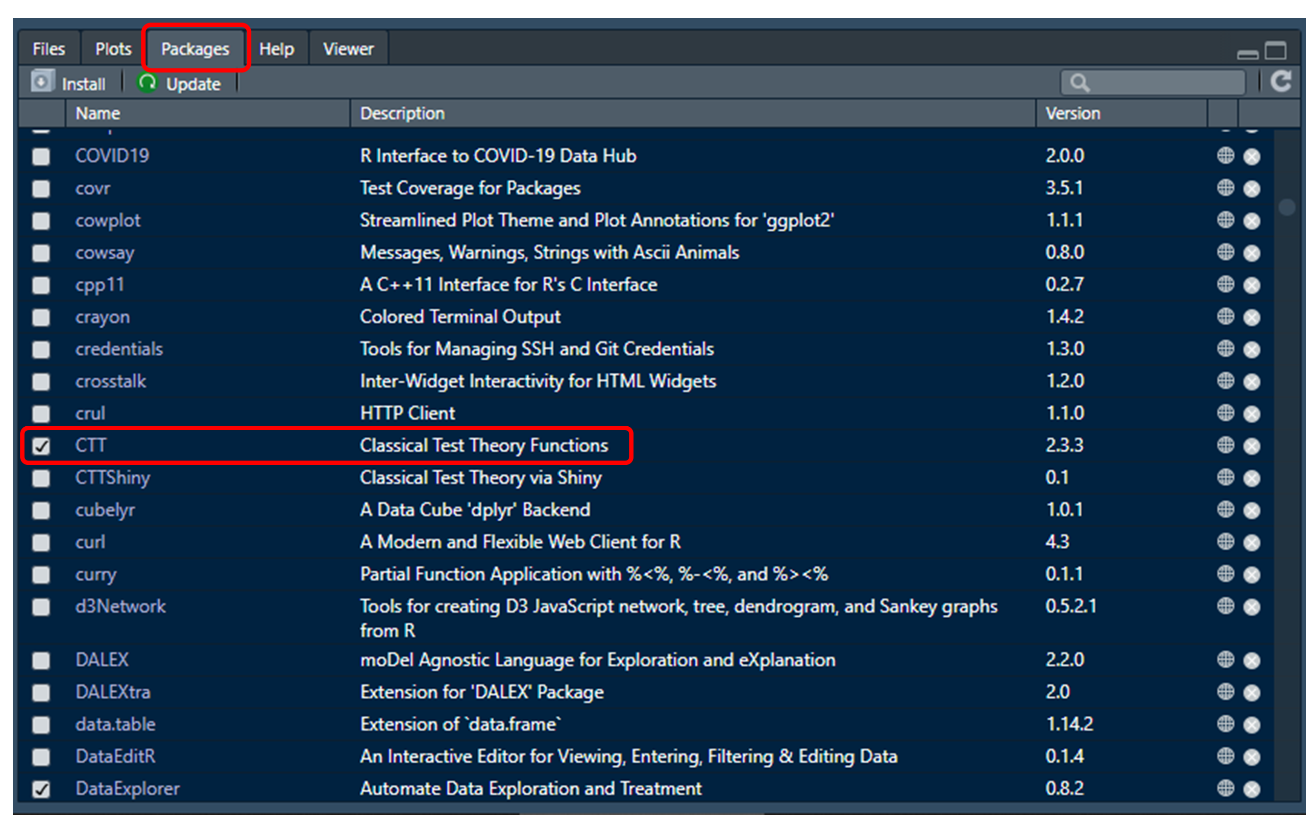
library("difR")Each of these packages comes with several functions. Once we activate a package, we can start using all the functions included in that package. To see what functions are included in a given package, we can go to “Miscellaneous” pane, click on the “Packages” menu option, find the package that we want to check on the list, and click on the package name to open its function directory. For example, we can click on the CTT package to see what functions are included in this package.
To call a particular function from a package, we need to know the
function name. For example, we can use the alpha() function
in the psych package to calculate internal consistency
values such as coefficient alpha. Since we are going to use multiple
functions from different packages, it might be a bit difficult to
remember which package each function comes from. Therefore, we will use
the following format in the codes: packagename::function.
For example, psych::alpha() indicates that we are calling
the alpha() function from the psych
package. If there is no “::” included in the function name (e.g.,
plot()), it means that we are using a built-in R function
(i.e., a function that comes with the base R).
🔔 INFORMATION: Using
::has two more benefits. First, when we use::, we can call a particular function from a package without activating the entire package. For example,psych::alpha()allows us to use thealpha()function without having to runlibrary("psych")beforehand. Second, if two or more packages activated within an R session include a function with the same name, then R only gives us access the function from the most recently activated package. This is called “masking”. For example, the ggplot2 package also has analpha()function. If we first loaded psych and then ggplot2, thealpha()from ggplot2 would mask thealpha()function from psych. However, by usingpsych::alpha(), we can still access thealpha()function from psych.
Exploratory data analysis
Exploratory data analysis (EDA) refers to the process of performing initial investigations on data in order to detect anomalies (e.g., unexpected values, high levels of missigness), check various assumptions (e.g., normality), and discover interesting patterns. When performing EDA, we often use both statistical and data visualization tools to summarize the data.
Before we begin the analysis, let’s set up our working directory. I created a new folder called “CTT Analysis” on my desktop and put our data (nfc_data.csv) into this folder. You can also create the same folder in a convenient location in your computer and save the path to this folder. Now, we can change our working directory to this new folder:
👍 SUGGESTION: We will use several datasets in the following examples. Downloading and putting all the data files into your working directory will make accessing these files easier.
Next, we will import the data into R. Since nfc_data.csv is a
comma-separated-values file (see the .csv extension), we will use the
read.csv() function to read our data into R and then save
it as “nfc”.
Using the head() function, we can now view the first 6
rows of the dataset:
Additionally, we can use View(nfc) that opens the data
viewer in RStudio and allows us to open the data in a spreadsheet-like
format.
  id age    sex education nfc01 nfc02 nfc03 nfc04 nfc05 nfc06 nfc07 nfc08 nfc09 nfc10 nfc11 nfc12 nfc13 nfc14
1  1  26   Male    Abitur     5     7     5     1     6     2     2     5     2     1     2     2     6     5
2  4  19 Female    Abitur     5     5     3     2     5     3     3     3     2     4     3     2     3     2
3  7  23 Female    Abitur     5     6     5     1     7     3     2     3     1     3     3     1     6     5
4  8  24 Female    Abitur     5     5     4     2     5     5     2     2     2     2     4     3     2     3
5 11  24 Female    Abitur     2     3     3     5     3     5     6     1     6     6     6     6     2     1
6 12  20 Female    Abitur     6     6     6     1     6     3     1     1     1     1     1     1     6     6
  nfc15 nfc16 action_orientation effortful_control self_control
1     2     1                 10                11            5
2     4     4                 11                32           16
3     1     1                 13                10           -2
4     1     1                  5                 0           -4
5     5     5                 18                10           11
6     2     2                 20                24           11
We can also see the names and types of the variables in our dataset
using the str() function (which shows us the
structure of the data):
'data.frame':   1209 obs. of  23 variables:
 $ id                : int  1 4 7 8 11 12 15 16 21 23 ...
 $ age               : int  26 19 23 24 24 20 25 27 21 25 ...
 $ sex               : chr  "Male" "Female" "Female" "Female" ...
 $ education         : chr  "Abitur" "Abitur" "Abitur" "Abitur" ...
 $ nfc01             : int  5 5 5 5 2 6 3 7 7 6 ...
 $ nfc02             : int  7 5 6 5 3 6 4 4 5 7 ...
 $ nfc03             : int  5 3 5 4 3 6 4 5 3 7 ...
 $ nfc04             : int  1 2 1 2 5 1 1 6 1 1 ...
 $ nfc05             : int  6 5 7 5 3 6 6 6 6 7 ...
 $ nfc06             : int  2 3 3 5 5 3 5 3 6 2 ...
 $ nfc07             : int  2 3 2 2 6 1 3 1 1 1 ...
 $ nfc08             : int  5 3 3 2 1 1 2 2 2 2 ...
 $ nfc09             : int  2 2 1 2 6 1 3 2 1 1 ...
 $ nfc10             : int  1 4 3 2 6 1 3 2 2 2 ...
 $ nfc11             : int  2 3 3 4 6 1 1 1 1 1 ...
 $ nfc12             : int  2 2 1 3 6 1 1 1 1 1 ...
 $ nfc13             : int  6 3 6 2 2 6 3 4 6 5 ...
 $ nfc14             : int  5 2 5 3 1 6 3 4 4 5 ...
 $ nfc15             : int  2 4 1 1 5 2 1 2 2 1 ...
 $ nfc16             : int  1 4 1 1 5 2 2 2 2 2 ...
 $ action_orientation: int  10 11 13 5 18 20 6 16 12 8 ...
 $ effortful_control : int  11 32 10 0 10 24 -3 2 -6 21 ...
 $ self_control      : int  5 16 -2 -4 11 11 -4 3 -10 5 ...
The dataset consists of 1209 rows (i.e., participants) and 23
variables (id, age, sex, education, nfc01 to nfc16 representing the
responses to the NFC Scale items, and three scores for criterion
measures). We can obtain a bit more information on the dataset using the
introduce() and plot_intro() functions from
the DataExplorer package (Cui,
2020):
| rows | 1,209 |
| columns | 23 |
| discrete_columns | 2 |
| continuous_columns | 21 |
| all_missing_columns | 0 |
| total_missing_values | 8 |
| complete_rows | 1,201 |
| total_observations | 27,807 |
| memory_usage | 126,664 |
The output above gives us a summary of our dataset with additional information on the total number of missing values, total number of observations, and so on.
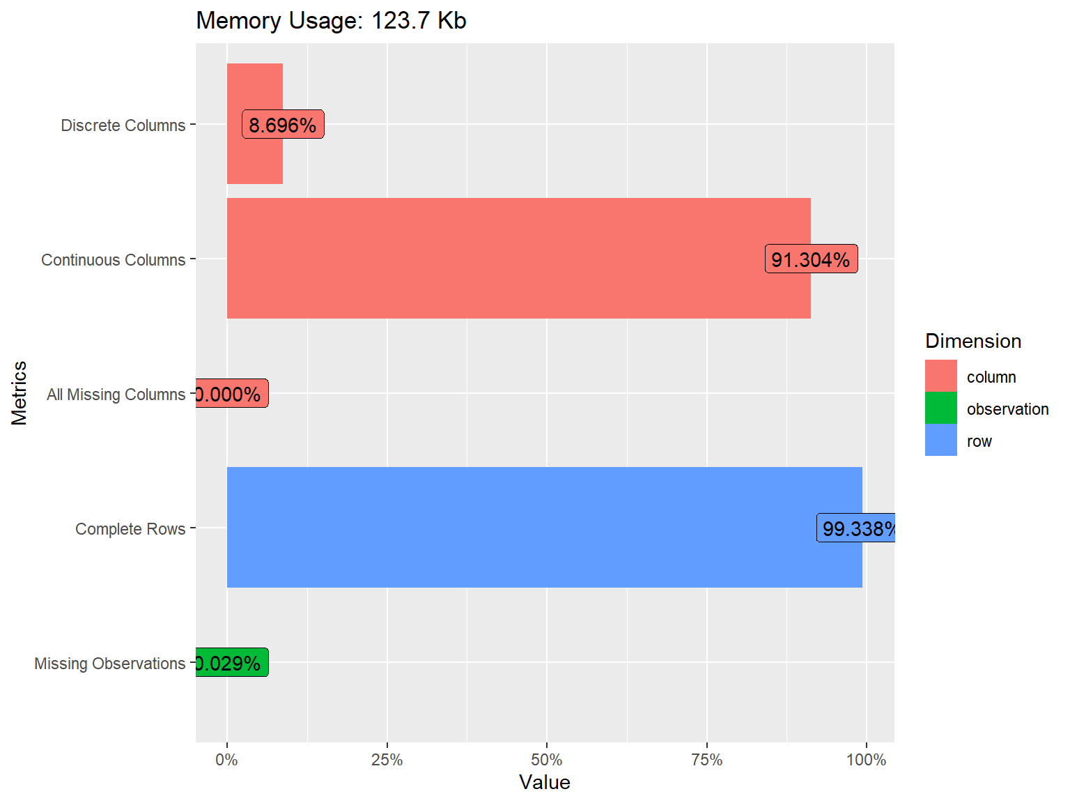
The plot above shows that most of the variables are continuous (note that R recognizes Likert-scale items as continuous variables although they are actually ordinal) while there are also some discrete (i.e., categorical) variables (i.e., sex and education) in the dataset. We also see that some of the variables in the dataset have missing values but the proportion of missing data is very small (only 0.023%). Depending on the sample size, missingness > 10% is often concerning as the loss of information due to these missing values is likely to influence the results of our analysis.
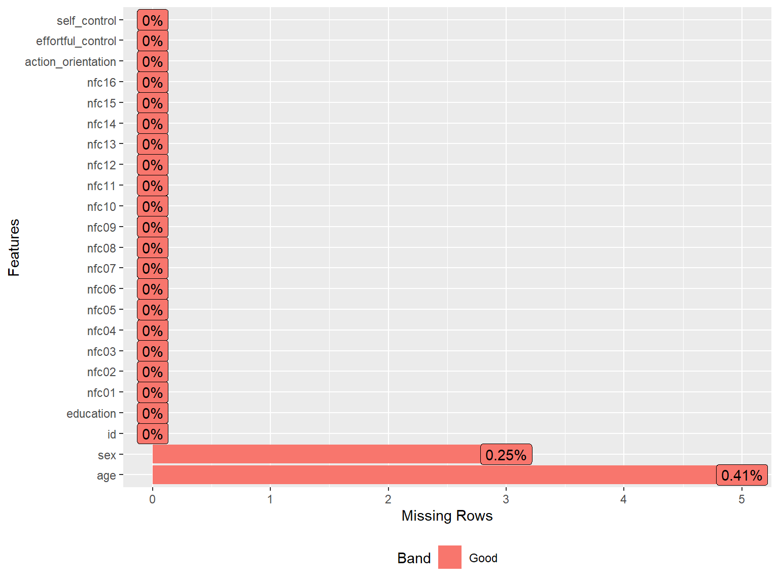
To have a closer look at missing values, we can visualize the proportion of missingness for each variable. The following plot shows that age and sex have some missing values but the proportion of missingness is very small (less than 1%).
The DataExplorer package also has additional functions to visualize both categorical and continuous variables. The package is using a simpler language to create plots based on the ggplot2 package (Wickham et al., 2021) in the background.
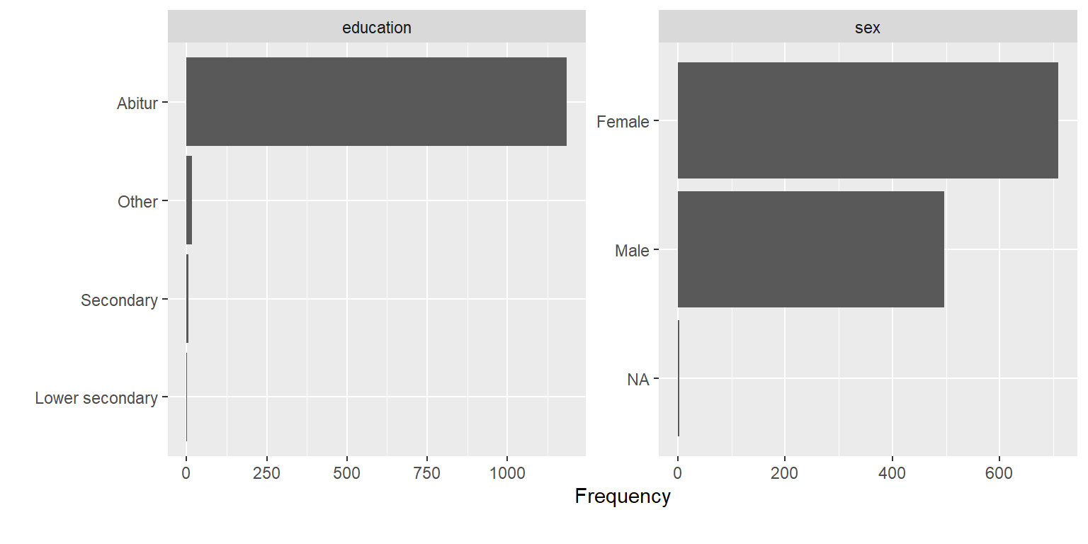
# Continuous variables (histogram)
DataExplorer::plot_histogram(data = nfc[, c("age", "self_control", "action_orientation", "effortful_control")])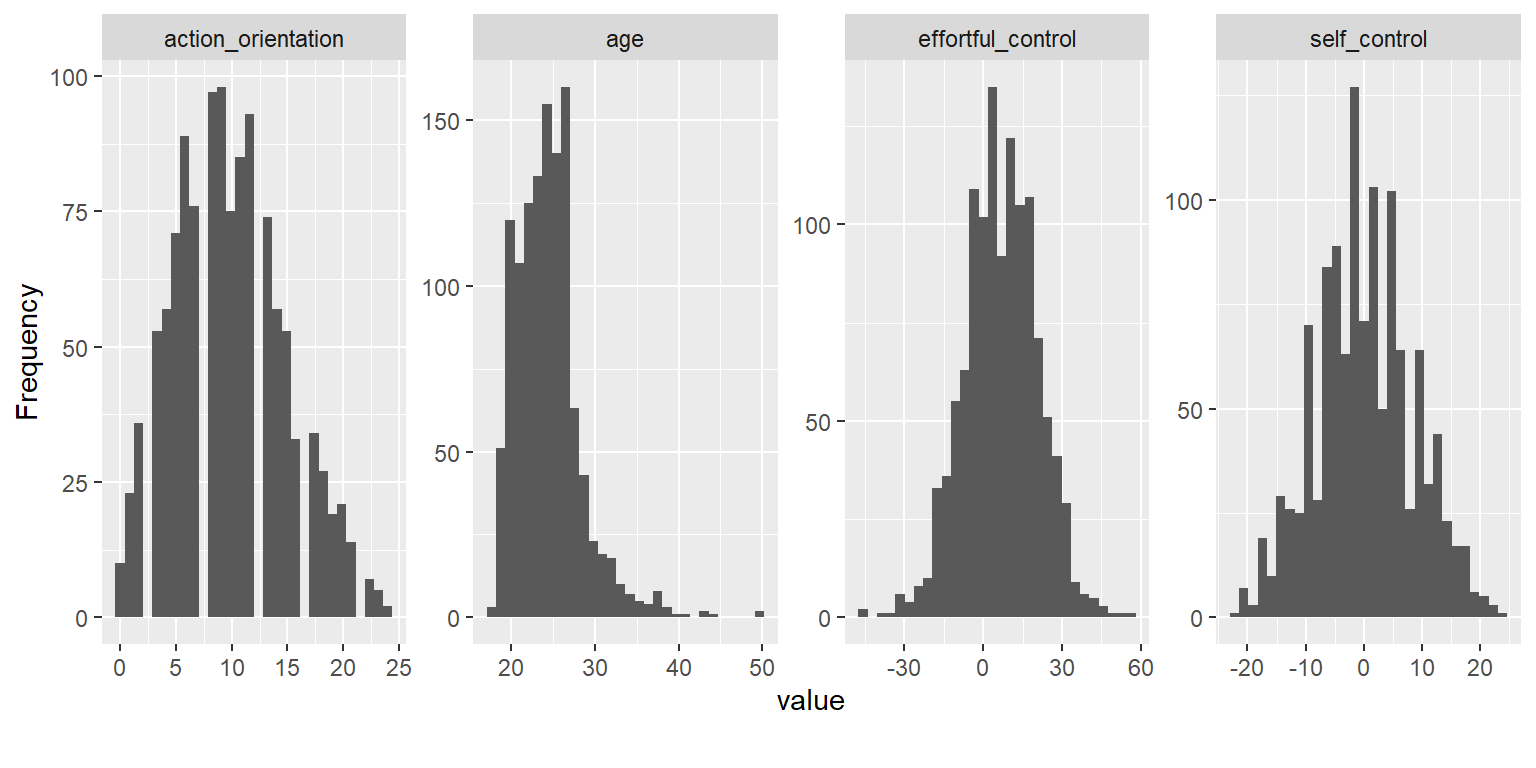
# Continuous variables (boxplot) by a categorical variable
DataExplorer::plot_boxplot(data = nfc[!is.na(nfc$sex), # select cases where sex is not missing
                                      # Select variables of interest
                                      c("sex", "self_control", "action_orientation", "effortful_control")],
                           by = "sex") # Draw boxplots by sex (a categorical variable)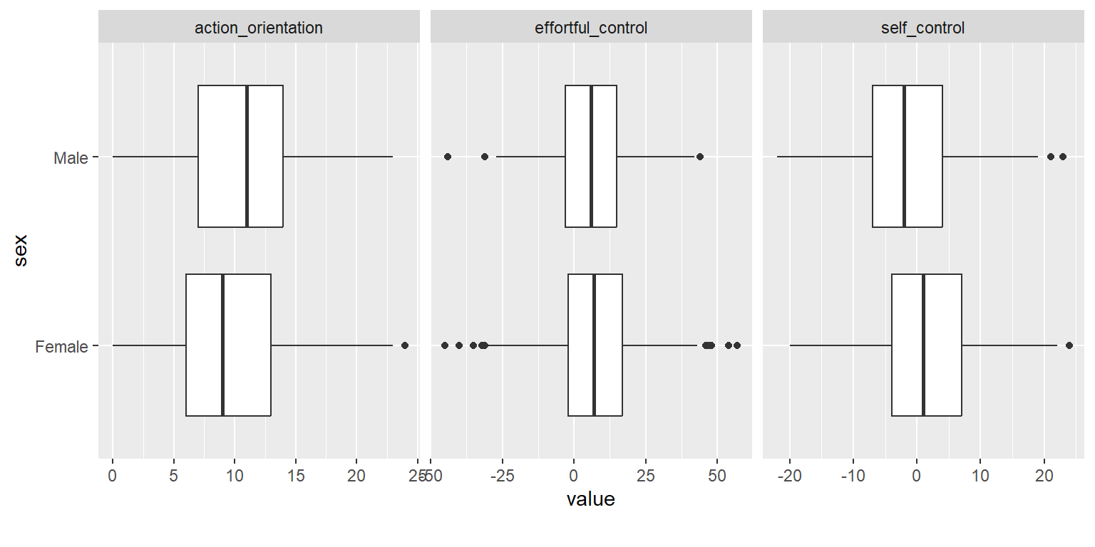
To organize all the summary statistics into a single report, we could
use the create_report() function. It runs most functions in
DataExplorer and outputs a HTML report file (assuming
rmarkdown has been already installed).
# Drop the id variable so it doesn't get analyzed with the other variables
nfc <- DataExplorer::drop_columns(nfc, "id")

# This code creates a report and saves it into the working directory
DataExplorer::create_report(data = nfc,
                            report_title = "NFC Scale Analysis",
                            output_file = "nfc_report.html")
To obtain a detailed summary of the nfc dataset within a single
analysis, we can use the skim() function from the
skimr package (Waring et al.,
2021). As you can see from the output below, we obtained similar
descriptive statistics for the variables in the nfc dataset:
- “Data Summary” shows the number of columns/rows and column types (i.e., variable types)
- “Variable type” tables show a summary of character (i.e., categorical) and numeric (i.e., continuous) variables
In “Variable type: character”, we see the number of missing values, complete data rate, the minimum number of characters (e.g., 4 for sex: male) and maximum number of characters (e.g., 6 for sex: female), and the number of unique values (e.g., 2 for sex: male and female) for the variables.
In “Variable type: numeric”, we see the number of missing values, complete data rate, mean, standard deviation, min (p0), 25th percentile (p25), median (p50), 75% percentile (p75), and max (p100) values for the variables.
── Data Summary ────────────────────────
                           Values
Name                       nfc
Number of rows             1209
Number of columns          23
_______________________
Column type frequency:
  character                2
  numeric                  21
________________________
Group variables            None

── Variable type: character ────────────────────────────────────────────────────────────────────────────────────────────────────────────────────────────────────────────────────────────────────────────
  skim_variable n_missing complete_rate min max empty n_unique whitespace
1 sex                   3         0.998   4   6     0        2          0
2 education             0         1       5  15     0        4          0

── Variable type: numeric ──────────────────────────────────────────────────────────────────────────────────────────────────────────────────────────────────────────────────────────────────────────────
   skim_variable      n_missing complete_rate    mean     sd  p0 p25 p50  p75 p100
 1 id                         0         1     882.    491.     1 464 888 1305 1735
 2 age                        5         0.996  24.4     3.93  18  22  24   26   50
 3 nfc01                      0         1       5.54    1.19   1   5   6    6    7
 4 nfc02                      0         1       4.94    1.39   1   4   5    6    7
 5 nfc03                      0         1       4.44    1.40   1   3   5    5    7
 6 nfc04                      0         1       2.47    1.47   1   1   2    3    7
 7 nfc05                      0         1       5.82    1.23   1   5   6    7    7
 8 nfc06                      0         1       3.75    1.50   1   3   4    5    7
 9 nfc07                      0         1       2.70    1.32   1   2   2    3    7
10 nfc08                      0         1       3.34    1.55   1   2   3    4    7
11 nfc09                      0         1       2.45    1.52   1   1   2    3    7
12 nfc10                      0         1       3.16    1.52   1   2   3    4    7
13 nfc11                      0         1       2.75    1.45   1   2   2    4    7
14 nfc12                      0         1       2.45    1.40   1   1   2    3    7
15 nfc13                      0         1       4.10    1.42   1   3   4    5    7
16 nfc14                      0         1       3.57    1.47   1   2   4    4    7
17 nfc15                      0         1       2.25    1.34   1   1   2    3    7
18 nfc16                      0         1       2.48    1.40   1   1   2    3    7
19 action_orientation         0         1       9.84    4.96   0   6   9   13   24
20 effortful_control          0         1       6.84   14.0  -45  -2   7   16   57
21 self_control               0         1       0.117   8.36 -22  -5   0    5   24
The describe() function from the psych
package (Revelle, 2021) is another useful
function to get basic descriptive statistics for data collected for
psychometric and psychology studies (see ?psych::describe
for more details about this function).
                   vars    n   mean     sd median trimmed    mad min  max range  skew kurtosis    se
id                    1 1209 881.61 490.93    888  883.82 624.17   1 1735  1734 -0.03    -1.18 14.12
age                   2 1204  24.43   3.93     24   24.00   2.97  18   50    32  1.54     4.79  0.11
sex*                  3 1206   1.41   0.49      1    1.39   0.00   1    2     1  0.36    -1.87  0.01
education*            4 1209   1.04   0.31      1    1.00   0.00   1    4     3  7.59    58.45  0.01
nfc01                 5 1209   5.54   1.19      6    5.68   1.48   1    7     6 -1.18     1.56  0.03
nfc02                 6 1209   4.94   1.39      5    5.01   1.48   1    7     6 -0.49    -0.31  0.04
nfc03                 7 1209   4.44   1.40      5    4.51   1.48   1    7     6 -0.32    -0.48  0.04
nfc04                 8 1209   2.47   1.47      2    2.25   1.48   1    7     6  1.16     0.68  0.04
nfc05                 9 1209   5.82   1.23      6    6.01   1.48   1    7     6 -1.33     2.09  0.04
nfc06                10 1209   3.75   1.50      4    3.69   1.48   1    7     6  0.24    -0.60  0.04
nfc07                11 1209   2.70   1.32      2    2.57   1.48   1    7     6  0.79     0.20  0.04
nfc08                12 1209   3.34   1.55      3    3.27   1.48   1    7     6  0.40    -0.65  0.04
nfc09                13 1209   2.45   1.52      2    2.23   1.48   1    7     6  1.03     0.32  0.04
nfc10                14 1209   3.16   1.52      3    3.06   1.48   1    7     6  0.61    -0.30  0.04
nfc11                15 1209   2.75   1.45      2    2.61   1.48   1    7     6  0.72    -0.15  0.04
nfc12                16 1209   2.45   1.40      2    2.26   1.48   1    7     6  0.93     0.18  0.04
nfc13                17 1209   4.10   1.42      4    4.13   1.48   1    7     6 -0.13    -0.54  0.04
nfc14                18 1209   3.57   1.47      4    3.54   1.48   1    7     6  0.11    -0.50  0.04
nfc15                19 1209   2.25   1.34      2    2.03   1.48   1    7     6  1.25     1.23  0.04
nfc16                20 1209   2.48   1.40      2    2.28   1.48   1    7     6  1.06     0.77  0.04
action_orientation   21 1209   9.84   4.96      9    9.65   4.45   0   24    24  0.33    -0.40  0.14
effortful_control    22 1209   6.84  13.97      7    6.93  13.34 -45   57   102 -0.08     0.27  0.40
self_control         23 1209   0.12   8.36      0    0.08   7.41 -22   24    46  0.06    -0.26  0.24
Before moving to item analysis, we should also check the correlations among the items to gauge how strongly the items are associated with each other. We expect the items to be associated with each other up to a certain degree because we assume that the items measure the same latent trait (the construct of NFC in this example). Having weakly-correlated items suggests that some items may not be measuring the same latent trait. Having very highly-correlated items (e.g., \(r > .95\)) suggests that there is some redundancy in the instrument because some items provide us with the same information about the individuals who answered the items.
In addition, we know that some items in the NFC Scale are negatively-worded and thus responses to these items may be in the opposite direction with the rest of the items. For example, individuals with high NFC are likely to choose “7 = completely agree” for a positively-worded item such as “Enjoyment of tasks that involve problem-solving” whereas they are expected to choose “1 = completely disagree” for a negatively-worded item such as “Anticipation and avoiding of situations that may require in-depth thinking”.
Now, we will create a correlation matrix of the NFC items and review
the strength and direction of the relationships among the items. First,
we will save the responses as a separate dataset to make our subsequent
analyses easier. The items in the nfc dataset are named as nfc01, nfc02,
…, nfc16. That is, they all start with the same prefix: nfc. So, we can
use this prefix to select the items more easily. We will use the
select() function from dplyr.
starts_with("nfc") will help us choose the variables
starting with “nfc” as a selection condition.
response <- dplyr::select(nfc, # name of the dataset
                          starts_with("nfc")) # variables to be selected

head(response)
nfc01 nfc02 nfc03 nfc04 nfc05 nfc06 nfc07 nfc08 nfc09 nfc10 nfc11 nfc12 nfc13
1 5 7 5 1 6 2 2 5 2 1 2 2 6
2 5 5 3 2 5 3 3 3 2 4 3 2 3
3 5 6 5 1 7 3 2 3 1 3 3 1 6
4 5 5 4 2 5 5 2 2 2 2 4 3 2
5 2 3 3 5 3 5 6 1 6 6 6 6 2
6 6 6 6 1 6 3 1 1 1 1 1 1 6
nfc14 nfc15 nfc16
1 5 2 1
2 2 4 4
3 5 1 1
4 3 1 1
5 1 5 5
6 6 2 2Alternatively, we could type each item by one one (which is much more tedious):
response <- dplyr::select(nfc, # name of the dataset
                          nfc01, nfc02, nfc03, nfc04, ..., nfc16) # variables to be selected
Next, we will compute the correlations among these items. Remember
that the NFC items follow an ordinal scale: 1=completely disagree to
7=completely agree. Therefore, instead of Pearson correlation (which can
be obtained using the cor() function in R), we will use the
polychoric() function from psych to
calculate polychoric correlations. The polychoric()
function produces several outcomes but we only want to keep
rho- (i.e., the correlation matrix of the items).
# Save the correlation matrix
cormat <- psych::polychoric(x = response)$rho

# Print the correlation matrix
print(cormat)| nfc01 | nfc02 | nfc03 | nfc04 | nfc05 | nfc06 | nfc07 | nfc08 | nfc09 | nfc10 | nfc11 | nfc12 | nfc13 | nfc14 | nfc15 | nfc16 | |
|---|---|---|---|---|---|---|---|---|---|---|---|---|---|---|---|---|
| nfc01 | 1.0000000 | 0.4902745 | 0.4206642 | -0.3100622 | 0.3664366 | -0.2129555 | -0.4443239 | -0.3682254 | -0.3348804 | -0.4170343 | -0.3979982 | -0.3301170 | 0.4784051 | 0.3739029 | -0.3168246 | -0.3645847 |
| nfc02 | 0.4902745 | 1.0000000 | 0.5586268 | -0.3518608 | 0.4302197 | -0.1714928 | -0.5024895 | -0.4101025 | -0.3043553 | -0.3396839 | -0.3501303 | -0.2940613 | 0.4328523 | 0.4344971 | -0.3412820 | -0.3391467 |
| nfc03 | 0.4206642 | 0.5586268 | 1.0000000 | -0.3285576 | 0.4036880 | -0.2341821 | -0.3956683 | -0.3289920 | -0.1764341 | -0.2570604 | -0.2960401 | -0.2650049 | 0.4211096 | 0.3674297 | -0.2462771 | -0.2068671 |
| nfc04 | -0.3100622 | -0.3518608 | -0.3285576 | 1.0000000 | -0.3525128 | 0.1755489 | 0.4340969 | 0.3819535 | 0.3273752 | 0.2870367 | 0.3533191 | 0.3746371 | -0.2351161 | -0.2095721 | 0.2878428 | 0.2236609 |
| nfc05 | 0.3664366 | 0.4302197 | 0.4036880 | -0.3525128 | 1.0000000 | -0.1670120 | -0.3831624 | -0.3043216 | -0.2884139 | -0.2200394 | -0.3305253 | -0.2572521 | 0.3158859 | 0.2573391 | -0.2913227 | -0.2208485 |
| nfc06 | -0.2129555 | -0.1714928 | -0.2341821 | 0.1755489 | -0.1670120 | 1.0000000 | 0.3214179 | 0.2003728 | 0.2179882 | 0.2964199 | 0.1882097 | 0.2165816 | -0.1894823 | -0.1342153 | 0.1524393 | 0.1891512 |
| nfc07 | -0.4443239 | -0.5024895 | -0.3956683 | 0.4340969 | -0.3831624 | 0.3214179 | 1.0000000 | 0.5226418 | 0.4446690 | 0.4498439 | 0.4896835 | 0.4943161 | -0.4082126 | -0.3530903 | 0.3762733 | 0.3402142 |
| nfc08 | -0.3682254 | -0.4101025 | -0.3289920 | 0.3819535 | -0.3043216 | 0.2003728 | 0.5226418 | 1.0000000 | 0.4514346 | 0.3984487 | 0.5124883 | 0.3659696 | -0.3531705 | -0.3338932 | 0.2992594 | 0.3034186 |
| nfc09 | -0.3348804 | -0.3043553 | -0.1764341 | 0.3273752 | -0.2884139 | 0.2179882 | 0.4446690 | 0.4514346 | 1.0000000 | 0.4039954 | 0.4915927 | 0.4466499 | -0.2520765 | -0.2129343 | 0.3017600 | 0.2611840 |
| nfc10 | -0.4170343 | -0.3396839 | -0.2570604 | 0.2870367 | -0.2200394 | 0.2964199 | 0.4498439 | 0.3984487 | 0.4039954 | 1.0000000 | 0.4075905 | 0.4707113 | -0.2951438 | -0.2215370 | 0.2306346 | 0.2640125 |
| nfc11 | -0.3979982 | -0.3501303 | -0.2960401 | 0.3533191 | -0.3305253 | 0.1882097 | 0.4896835 | 0.5124883 | 0.4915927 | 0.4075905 | 1.0000000 | 0.4316886 | -0.3984187 | -0.3468447 | 0.2793425 | 0.2887587 |
| nfc12 | -0.3301170 | -0.2940613 | -0.2650049 | 0.3746371 | -0.2572521 | 0.2165816 | 0.4943161 | 0.3659696 | 0.4466499 | 0.4707113 | 0.4316886 | 1.0000000 | -0.2978599 | -0.2043646 | 0.2973833 | 0.2840847 |
| nfc13 | 0.4784051 | 0.4328523 | 0.4211096 | -0.2351161 | 0.3158859 | -0.1894823 | -0.4082126 | -0.3531705 | -0.2520765 | -0.2951438 | -0.3984187 | -0.2978599 | 1.0000000 | 0.6012045 | -0.2304441 | -0.2548785 |
| nfc14 | 0.3739029 | 0.4344971 | 0.3674297 | -0.2095721 | 0.2573391 | -0.1342153 | -0.3530903 | -0.3338932 | -0.2129343 | -0.2215370 | -0.3468447 | -0.2043646 | 0.6012045 | 1.0000000 | -0.2058702 | -0.1995835 |
| nfc15 | -0.3168246 | -0.3412820 | -0.2462771 | 0.2878428 | -0.2913227 | 0.1524393 | 0.3762733 | 0.2992594 | 0.3017600 | 0.2306346 | 0.2793425 | 0.2973833 | -0.2304441 | -0.2058702 | 1.0000000 | 0.7530236 |
| nfc16 | -0.3645847 | -0.3391467 | -0.2068671 | 0.2236609 | -0.2208485 | 0.1891512 | 0.3402142 | 0.3034186 | 0.2611840 | 0.2640125 | 0.2887587 | 0.2840847 | -0.2548785 | -0.1995835 | 0.7530236 | 1.0000000 |
One thing that we can see right away is negative values in the
correlation matrix, confirming that some items are indeed negatively
correlated with each other. However, reviewing the rest of this 16x16
correlation matrix is not necessarily easy. We can’t just eyeball the
values to evaluate the associations among the items. Therefore, we will
create a correlation matrix plot using the ggcorrplot
package (Kassambara, 2019). The package
has a function with the same name, ggcorrplot(), that
transforms a correlation matrix into a nice correlation matrix plot
(note that a similar plot can be created using corPlot()
from psych).
ggcorrplot::ggcorrplot(corr = cormat, # correlation matrix
                       type = "lower", # print only the lower part of the correlation matrix
                       show.diag = TRUE, # show the diagonal values of 1
                       lab = TRUE, # add correlation values as labels
                       lab_size = 3) # Size of the labels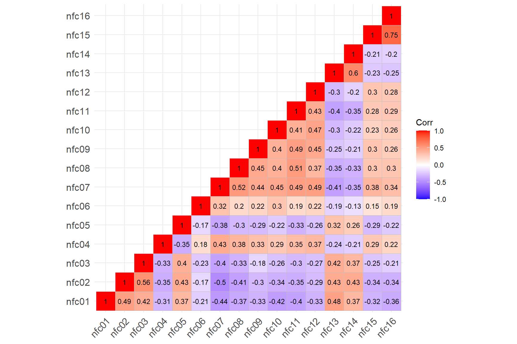
There are tons of options to customize the correlation matrix plot
(run ?ggcorrplot::ggcorrplot to see the help page), but
this is already a very good visualization for us to evaluate the
correlations among the items. We see that several items on the scale
(see the blue-coloured boxes) are negatively correlated with the rest of
the items. These are the (R) marked items in the NFC Scale (i.e.,
negatively-worded items). We will go ahead and reverse-code the
responses to these items (i.e., 1=completely agree to 7=completely
disagree) to put all the items in the same direction.
We will use the reverse.code() function from
psych for this process. We will create a reverse-coding
key where “1” keeps the item the same and “-1” reverse-codes the item.
In nfc_key below, we type “1” three times (no
reverse-coding for the first three items), type “-1” for the 4th item
(reverse-code the item), type 1 for the 5th item (no reverse-coding),
and so on. That is, the values in nfc_key correspond to the
positions of the items in the response dataset. Then, we
use reverse.code() to apply the key and transform the data
(saved as response_recoded).
# -1 means reverse-code the item
nfc_key <- c(1,1,1,-1,1,-1,-1,-1,-1,-1,-1,-1,1,1,-1,-1)

response_recoded <- psych::reverse.code(
  keys = nfc_key, # reverse-coding key
  items = response, # dataset to be transformed
  mini = 1, # minimum response value
  maxi = 7) # maximum response value
Let’s see if our transformation worked:
cormat_recoded <- psych::polychoric(response_recoded)$rho

ggcorrplot::ggcorrplot(corr = cormat_recoded,
                       type = "lower",
                       show.diag = TRUE,
                       lab = TRUE,
lab_size = 3) 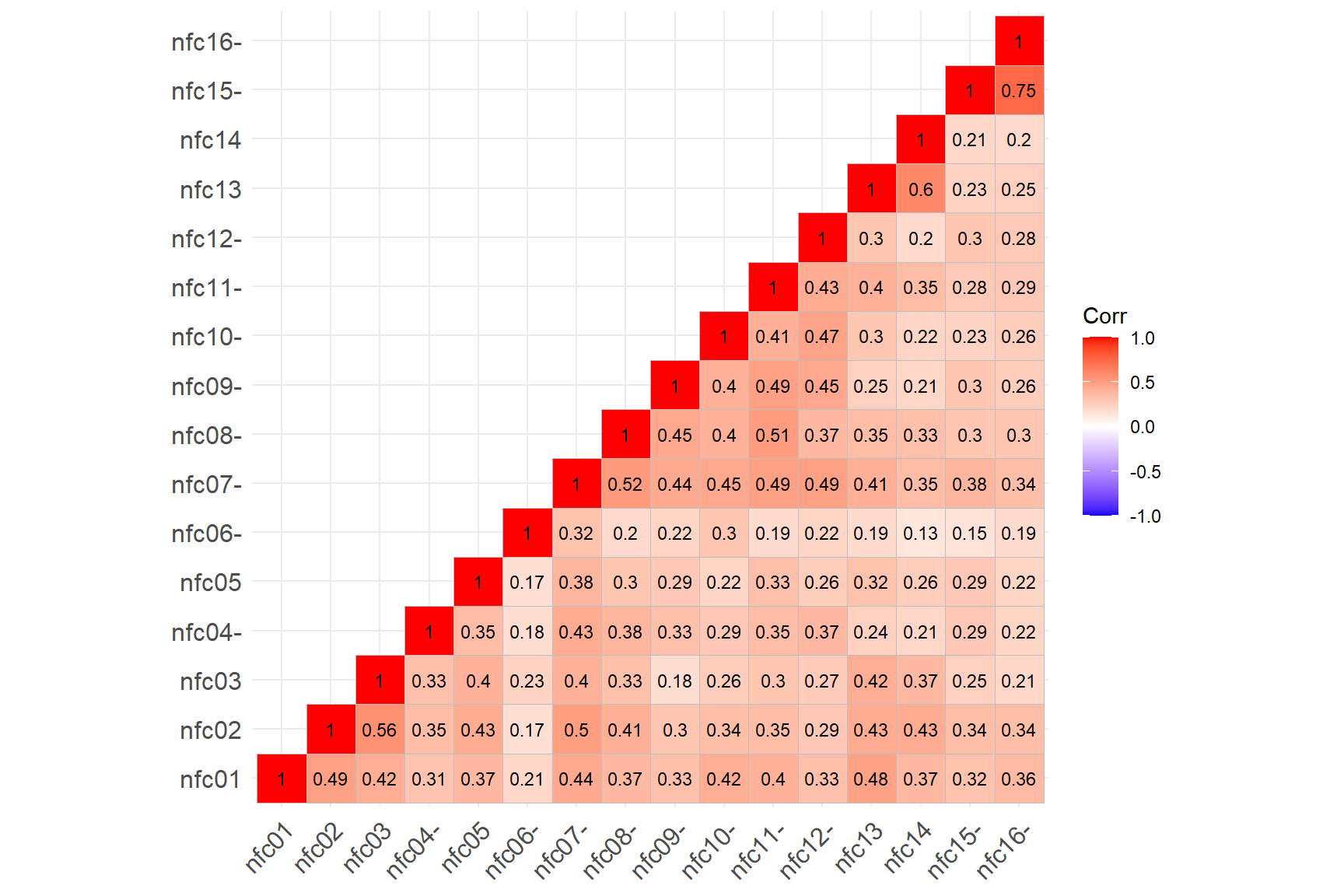
We can see in the correlation matrix plot that all the items are now
positively correlated with each other. Most correlations are moderate
while there also some items (e.g., nfc06) that seem to have low
correlations with the other items in the NFC scale. Also, we see that
reverse.code() changed the names of the reverse-coded items
by include “-” at the end (e.g., nfc04-). This is not necessarily a
problem. However, if we want to keep the original variable names (i.e.,
nfc01 to nfc16), we can rename the column names using the
colnames() function. The following will replace the column
names of the transformed data (i.e., response_recoded) with
the column names of the original response data (i.e.,
response) and then save the dataset as a data frame (the
typical data format in R).
# Rename the columns
colnames(response_recoded) <- colnames(response)

# Save the data as a data frame
response_recoded <- as.data.frame(response_recoded)

# Preview the first six rows of the data
head(response_recoded)
nfc01 nfc02 nfc03 nfc04 nfc05 nfc06 nfc07 nfc08 nfc09 nfc10 nfc11 nfc12 nfc13 nfc14 nfc15 nfc16
1 5 7 5 7 6 6 6 3 6 7 6 6 6 5 6 7
2 5 5 3 6 5 5 5 5 6 4 5 6 3 2 4 4
3 5 6 5 7 7 5 6 5 7 5 5 7 6 5 7 7
4 5 5 4 6 5 3 6 6 6 6 4 5 2 3 7 7
5 2 3 3 3 3 3 2 7 2 2 2 2 2 1 3 3
6 6 6 6 7 6 5 7 7 7 7 7 7 6 6 6 6Item analysis
Item analysis refers to the analysis of individual items on a measurement instrument in terms of descriptive statistics (e.g., mean, standard deviation, min, and max), item-level statistics (e.g., difficulty and discrimination), and their associations with scale-level statistics (e.g., reliability). In R, there are several packages to conduct item analysis on dichotomous items (i.e., 0 or 1) and ordinal items (e.g., Likert-scale items). I will demonstrate three of these packages below:
CTT (Willse, 2018):
The itemAnalysis() function runs item analysis and returns
a brief but useful table of item statistics. Specifying the dataset to
be analyzed (response_recoded) in the itemAnalysis()
function is enough to run item analysis. In the following example, we
will also set two flags for point-biserial correlation (pBisFlag) and
biserial correlation (bisFlag). Both of these statistics indicate the
discriminatory power of the items. In practice, we prefer both
point-biserial correlation and biserial correlation values to be at
least 0.2 or larger. So, we will set the flag at 0.2 so that the
function shows us (using an “X” sign) the items with discrimination of
.2 or less (see more details on the help page via
?CTT::itemAnalysis).
# Run the item analysis and save it as itemanalysis_ctt
itemanalysis_ctt <- CTT::itemAnalysis(items = response_recoded, pBisFlag = .2, bisFlag = .2)

# Print the item report
itemanalysis_ctt$itemReport
itemName itemMean pBis bis alphaIfDeleted lowPBis lowBis
1 nfc01 5.535153 0.5830007 0.6324858 0.8603155
2 nfc02 4.944582 0.5983857 0.6212552 0.8587924
3 nfc03 4.435897 0.5120628 0.5278773 0.8626385
4 nfc04 5.526882 0.4275829 0.4678823 0.8665634
5 nfc05 5.818859 0.4657545 0.5132235 0.8646917
6 nfc06 4.254756 0.3164060 0.3254804 0.8717944
7 nfc07 5.299421 0.6637826 0.7012827 0.8562648
8 nfc08 4.660050 0.5697411 0.5895616 0.8598588
9 nfc09 5.549214 0.4916520 0.5349076 0.8636576
10 nfc10 4.837055 0.5032326 0.5251349 0.8631153
11 nfc11 5.254756 0.5772984 0.6088347 0.8596070
12 nfc12 5.554177 0.5069643 0.5468089 0.8628642
13 nfc13 4.104218 0.5384126 0.5524339 0.8614377
14 nfc14 3.570720 0.4585722 0.4710690 0.8651300
15 nfc15 5.752688 0.4678062 0.5152649 0.8645620
16 nfc16 5.524400 0.4585389 0.4943813 0.8650091 In the output above, “itemMean” is the average response value for each item (which is not necessarily useful given that our items are ordinal), “pBis” and “bis” refer to point-biserial and bi-serial correlations respectively, “alphaIfDeleted” indicates how the reliability of the instrument would change if each item were to be removed (we will discuss reliability in the next section), and the last two columns (“lowPBis” and “lowBis”) are the columns where we would see flags (i.e., X marks) if the values are less than 0.2. In this example, all the items seem to have pBis and bis values larger than 0.2 and thus there are no flagged items.
psych (Revelle, 2021):
The alpha() function runs item analysis and returns a
detailed output with both item-level and scale-level statistics. To use
the function, we need to specify the response dataset to be analyzed
(i.e., x = response_recoded). The function also involves
other arguments (e.g., na.rm = TRUE to remove missing
values and find pairwise correlations), but the default values for these
arguments are sufficient to conduct item analysis (see more details on
the help page via ?psych::alpha).
# Run the item analysis and save it as itemanalysis_psych
itemanalysis_psych <- psych::alpha(x = response_recoded)

# Print the results
itemanalysis_psych
Reliability analysis
Call: psych::alpha(x = response_recoded)

  raw_alpha std.alpha G6(smc) average_r S/N    ase mean   sd median_r
      0.87      0.87    0.88       0.3 6.8 0.0054    5 0.82     0.29

    95% confidence boundaries
         lower alpha upper
Feldt     0.86  0.87  0.88
Duhachek  0.86  0.87  0.88

 Reliability if an item is dropped:
      raw_alpha std.alpha G6(smc) average_r S/N alpha se  var.r med.r
nfc01      0.86      0.86    0.87      0.29 6.2   0.0059 0.0098  0.27
nfc02      0.86      0.86    0.87      0.29 6.2   0.0059 0.0091  0.28
nfc03      0.86      0.86    0.88      0.30 6.4   0.0058 0.0094  0.29
nfc04      0.87      0.87    0.88      0.31 6.6   0.0056 0.0098  0.30
nfc05      0.86      0.87    0.88      0.30 6.5   0.0057 0.0100  0.30
nfc06      0.87      0.87    0.89      0.31 6.9   0.0054 0.0084  0.31
nfc07      0.86      0.86    0.87      0.29 6.0   0.0060 0.0092  0.27
nfc08      0.86      0.86    0.88      0.29 6.3   0.0059 0.0098  0.28
nfc09      0.86      0.87    0.88      0.30 6.4   0.0057 0.0097  0.30
nfc10      0.86      0.87    0.88      0.30 6.4   0.0058 0.0099  0.29
nfc11      0.86      0.86    0.87      0.29 6.2   0.0059 0.0096  0.28
nfc12      0.86      0.87    0.88      0.30 6.4   0.0058 0.0098  0.29
nfc13      0.86      0.86    0.87      0.30 6.3   0.0058 0.0091  0.29
nfc14      0.87      0.87    0.88      0.30 6.5   0.0057 0.0088  0.29
nfc15      0.86      0.87    0.87      0.30 6.5   0.0057 0.0084  0.30
nfc16      0.87      0.87    0.87      0.30 6.5   0.0057 0.0083  0.30

 Item statistics
         n raw.r std.r r.cor r.drop mean  sd
nfc01 1209  0.64  0.65  0.62   0.58  5.5 1.2
nfc02 1209  0.66  0.67  0.65   0.60  4.9 1.4
nfc03 1209  0.59  0.59  0.56   0.51  4.4 1.4
nfc04 1209  0.52  0.51  0.46   0.43  5.5 1.5
nfc05 1209  0.54  0.55  0.50   0.47  5.8 1.2
nfc06 1209  0.42  0.41  0.34   0.32  4.3 1.5
nfc07 1209  0.72  0.72  0.70   0.66  5.3 1.3
nfc08 1209  0.65  0.64  0.61   0.57  4.7 1.6
nfc09 1209  0.58  0.57  0.53   0.49  5.5 1.5
nfc10 1209  0.59  0.58  0.54   0.50  4.8 1.5
nfc11 1209  0.65  0.64  0.62   0.58  5.3 1.4
nfc12 1209  0.58  0.58  0.54   0.51  5.6 1.4
nfc13 1209  0.61  0.61  0.59   0.54  4.1 1.4
nfc14 1209  0.54  0.54  0.51   0.46  3.6 1.5
nfc15 1209  0.55  0.55  0.53   0.47  5.8 1.3
nfc16 1209  0.54  0.54  0.53   0.46  5.5 1.4

Non missing response frequency for each item
         1    2    3    4    5    6    7 miss
nfc01 0.01 0.02 0.05 0.07 0.25 0.43 0.18    0
nfc02 0.01 0.05 0.10 0.18 0.27 0.26 0.12    0
nfc03 0.02 0.08 0.15 0.22 0.29 0.19 0.05    0
nfc04 0.01 0.05 0.06 0.08 0.15 0.37 0.28    0
nfc05 0.01 0.02 0.03 0.06 0.21 0.33 0.34    0
nfc06 0.04 0.11 0.14 0.27 0.21 0.19 0.05    0
nfc07 0.01 0.03 0.07 0.14 0.24 0.35 0.17    0
nfc08 0.02 0.08 0.13 0.18 0.24 0.23 0.11    0
nfc09 0.02 0.03 0.07 0.11 0.15 0.28 0.34    0
nfc10 0.03 0.06 0.12 0.15 0.25 0.28 0.12    0
nfc11 0.01 0.04 0.09 0.13 0.22 0.30 0.21    0
nfc12 0.01 0.02 0.09 0.09 0.18 0.32 0.30    0
nfc13 0.04 0.11 0.19 0.25 0.25 0.13 0.04    0
nfc14 0.09 0.16 0.21 0.29 0.15 0.07 0.03    0
nfc15 0.01 0.02 0.05 0.07 0.17 0.32 0.36    0
nfc16 0.01 0.03 0.06 0.08 0.22 0.31 0.28    0
The first part of the output shows the results of reliability analysis but we will discuss these results in the next section. For now, let’s focus on “Item statistics” and “Non missing response frequency for each item”.
Item statistics: The table shows the number of valid responses for each item (n), correlations between the items and the total score from the instrument (raw.r) where the item itself is included in the calculation of the total score, correlations between the items and the total score if the items were all standardized (std.r), correlations between the items and the total score corrected for both item overlap and scale reliability (r.cor), correlations between the items and the total score where the item of interest is not included in the calculation of the total score (r.drop), average response values (mean), and standard deviation of response values (sd). Compared with raw.r, r.cor and r.drop are better indicators of item discrimination as they indicate the relationship between each item and the rest of the items without contaminating the total score. We want r.cor and r.drop values to be larger than 0.2 for each item.
Non missing response frequency for each item: The table shows what percentages of respondents selected each response option of the each of the items. Each item in the NFC Scale have response options of 1 to 7 and thus we see each of these response options and the missing response in the last column. This table helps us check the distribution of response options and whether all or almost all respondents selected the same response options for some items (which lowers the reliability). In our example, we can see that the lowest response option (i.e., 1) was selected by a very low proportion of respondents whereas the middle and upper response categories (i.e., 4, 5, 6, and 7) were selected by much more respondents.
ShinyItemAnalysis (Martinkova
et al., 2021): The ItemAnalysis() function runs item
analysis and returns much more detailed output compared with those of
CTT and psych. The function has so
many options that allows users to customize the item analysis report in
several ways (see more details on the help page via
?ShinyItemAnalysis::ItemAnalysis). Also, using the
startShinyItemAnalysis() function, we can use the
interactive version of ItemAnalysis() where we can import
the data and select the analysis to be conducted using a nice user
interface based on the shiny package (for examples of
interesting shiny applications, see https://shiny.rstudio.com/).
# Run the item analysis and save it as itemanalysis_shiny
itemanalysis_shiny <- ShinyItemAnalysis::ItemAnalysis(Data = response_recoded)

# Print the results
itemanalysis_shiny
Difficulty Mean SD Cut.score obs.min Min.score obs.max Max.score Prop.max.score RIR
nfc01 0.7558588 5.535153 1.188645 NA 1 1 7 7 0.17866005 0.5830007
nfc02 0.6574304 4.944582 1.390390 NA 1 1 7 7 0.12406948 0.5983857
nfc03 0.5726496 4.435897 1.396922 NA 1 1 7 7 0.04962779 0.5120628
nfc04 0.7544803 5.526882 1.473097 NA 1 1 7 7 0.27791563 0.4275829
nfc05 0.8031431 5.818859 1.227220 NA 1 1 7 7 0.34491315 0.4657545
nfc06 0.5424593 4.254756 1.499872 NA 1 1 7 7 0.04797353 0.3164060
nfc07 0.7165702 5.299421 1.318365 NA 1 1 7 7 0.17038875 0.6637826
nfc08 0.6100083 4.660050 1.554549 NA 1 1 7 7 0.10918114 0.5697411
nfc09 0.7582024 5.549214 1.515188 NA 1 1 7 7 0.33995037 0.4916520
nfc10 0.6395092 4.837055 1.524876 NA 1 1 7 7 0.11579818 0.5032326
nfc11 0.7091260 5.254756 1.448205 NA 1 1 7 7 0.21339950 0.5772984
nfc12 0.7590295 5.554177 1.399119 NA 1 1 7 7 0.29859388 0.5069643
nfc13 0.5173697 4.104218 1.420891 NA 1 1 7 7 0.03639371 0.5384126
nfc14 0.4284533 3.570720 1.471642 NA 1 1 7 7 0.02564103 0.4585722
nfc15 0.7921147 5.752688 1.344924 NA 1 1 7 7 0.35649297 0.4678062
nfc16 0.7540667 5.524400 1.402319 NA 1 1 7 7 0.27956989 0.4585389
RIT Corr.criterion ULI gULI Alpha.drop Index.rel Index.val Perc.miss Perc.nr
nfc01 0.6409212 NA 0.2726639 NA 0.8603155 0.7618279 NA 0 0
nfc02 0.6639133 NA 0.3391863 NA 0.8587924 0.9230985 NA 0 0
nfc03 0.5880748 NA 0.3049003 NA 0.8626385 0.8214949 NA 0 0
nfc04 0.5166594 NA 0.2873591 NA 0.8665634 0.7610891 NA 0 0
nfc05 0.5370291 NA 0.2271560 NA 0.8646917 0.6590526 NA 0 0
nfc06 0.4168850 NA 0.2222994 NA 0.8717944 0.6252740 NA 0 0
nfc07 0.7178357 NA 0.3415068 NA 0.8562648 0.9463698 NA 0 0
nfc08 0.6466604 NA 0.3888922 NA 0.8598588 1.0052654 NA 0 0
nfc09 0.5762896 NA 0.3239544 NA 0.8636576 0.8731874 NA 0 0
nfc10 0.5870436 NA 0.3259830 NA 0.8631153 0.8951689 NA 0 0
nfc11 0.6481750 NA 0.3536981 NA 0.8596070 0.9386902 NA 0 0
nfc12 0.5836499 NA 0.2986357 NA 0.8628642 0.8165957 NA 0 0
nfc13 0.6126837 NA 0.3263285 NA 0.8614377 0.8705567 NA 0 0
nfc14 0.5444198 NA 0.3143888 NA 0.8651300 0.8011912 NA 0 0
nfc15 0.5455510 NA 0.2594773 NA 0.8645620 0.7337244 NA 0 0
nfc16 0.5404478 NA 0.2721719 NA 0.8650091 0.7578802 NA 0 0In the output above, there is tons of information regarding the items, but the ones we will focus on include:
- Difficulty: A standardized difficulty value between 0 and 1 based on the average score of the item divided by its range
- Mean: Average item score (again, not very useful for ordinal items)
- SD: Standard deviation of item scores
- RIT: Correlations between item scores and the total test score (same as r.raw from psych)
- RIR: Correlations between item scores and the total test score without the given item (same as r.drop from psych)
The ShinyItemAnalysis package also includes a
DDplot() function to visualize standardized difficulty and
discrimination statistics together. For the discrim
argument, we will use “RIR” to plot corrected item
discrimination values (alternatively, we could use “RIT” for uncorrected
discrimination values or “none” to plot only difficulty values).
# Create a difficulty and discrimination (DD) plot
ShinyItemAnalysis::DDplot(Data = response_recoded, discrim = "RIR")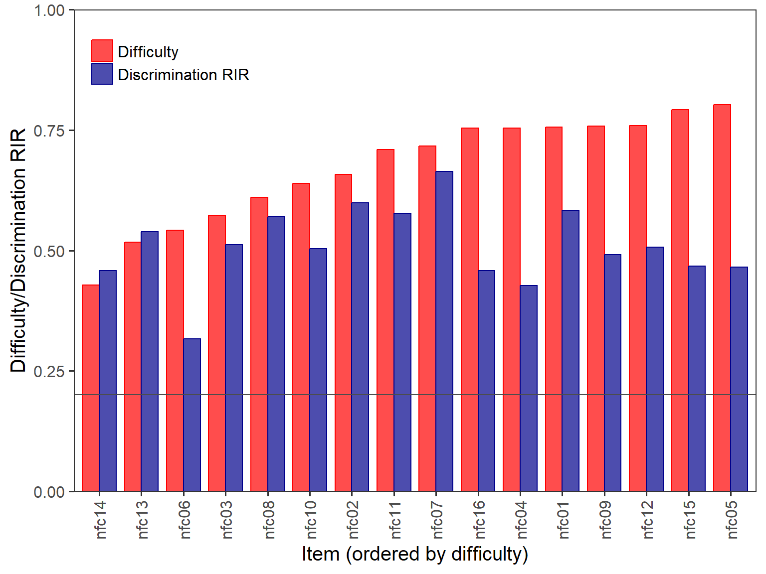
Reliability
Split-half reliability
As a simple measure of reliability, split-half reliability can be
obtained by splitting a measurement instrument into two equivalent
halves, calculating the total scores on the two halves, and correlating
them. There are several ways to create the split-half (e.g., selecting
every other items, randomly, etc.). Below, we will define a custom R
function to calculate the split-half reliability (this function
originally comes from the hemp
package). To create the split-half, we can choose either
type = "alternate" to select every other item (i.e., odd
and even numbered items) or type == "random" to select two
sets of items randomly. The seed argument is just an
integer for us to control random sampling if we choose
type == "random". Changing the seed will allow us to sample
a different set of items when we run the function every time.
split_half <- function(data, type = "alternate", seed = 2022) {

  # Select every other item
  if (type == "alternate") {
    first_half <- data[, seq(1, ncol(data), by = 2)]
    second_half <- data[, seq(2, ncol(data), by = 2)]
    first_total <- rowSums(first_half, na.rm = T)
    second_total <- rowSums(second_half, na.rm = T)
    rel <- round(cor(first_total, second_total), 3)} else

  # Select two halves randomly
  if (type == "random") {
    set.seed(seed)
    num_items <- 1:ncol(data)
    first_items <- sample(num_items, round(ncol(data)/2, 0))
    first_half <- data[, first_items]
    second_half <- data[, -first_items]
    first_total <- rowSums(first_half, na.rm = T)
    second_total <- rowSums(second_half, na.rm = T)
    rel <- round(cor(first_total, second_total), 3)}

  return(rel)
}
Now, let’s see what the split_half() function gives us
for the NFC Scale:
[1] 0.807[1] 0.826By changing the seed, we can run the split_half()
function many times, obtain a sample of split-half reliability
estimates, and find the average of these estimates as our final
split-half reliability value. Luckily, this process is much easier with
splitHalf() function in the psych package.
This functions calculates all (or at least a large number of) possible
split-half reliability values for a given dataset. Only specifying the
dataset to be analyzed is sufficient to use this function.
Split half reliabilities
Call: psych::splitHalf(r = response_recoded)

Maximum split half reliability (lambda 4) =  0.92
Guttman lambda 6                          =  0.88
Average split half reliability            =  0.87
Guttman lambda 3 (alpha)                  =  0.87
Guttman lambda 2                          =  0.88
Minimum split half reliability  (beta)    =  0.78
Average interitem r =  0.3  with median =  0.29
In the output above, we see that the minimum and maximum split-half
reliability estimates are 0.78 and 0.92, respectively. The output also
reports the average values of all split-half reliability estimates as
0.87. Now, let’s take a closer look at the split-half reliability
estimates we obtained for the NFC Scale. Using the
raw = TRUE argument, we will save all the split-half
reliability values and then visualize them using a histogram (with
hist()). The following histogram shows how the split-half
reliability estimates the NFC scale vary.
# Save the reliability results as sp_rel
sp_rel <- psych::splitHalf(r = response_recoded, raw = TRUE)

hist(x = sp_rel$raw, # extract the raw reliability values saved in sp_rel
     breaks = 101, # the number of breakpoints between histogram cells
     xlab = "Split-Half Reliability", # label for the x-axis
     main = "All Split-Half Reliabilities for the NFC Scale") # title for the histogram

# Add a red, vertical line showing the mean
# here v is a (v)ertical line
# col is the colour of the line
# lwd is the width of the line (the larger, the thicker line)
# lty is the line type (1 = solid, 2 = dashed, etc.)
# See http://www.sthda.com/english/wiki/line-types-in-r-lty for more details
abline(v = mean(sp_rel$raw), col = "red", lwd = 2, lty = 2)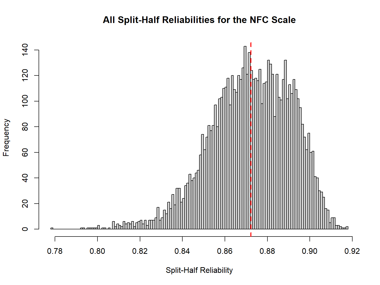
Internal consistency
Next, we will calculate internal consistency, more specifically coefficient alpha (NOT Cronbach’s alpha), for the NFC Scale. Internal consistency is the degree of homogeneity among the items on a measurement instrument. It allows us to gauge how strongly the items in a given instrument are associated with each other. A common misconception about internal consistency is that coefficient alpha and its variants can tell us how well a measurement instrument is actually measuring what we want it to measure, which is INCORRECT. If the items measure the same target construct (which may not necessarily be what we wanted to measure), then they are expected to be internally consistent with one another (i.e., correlated) and yield reliable (i.e., consistent) results.
There are multiple ways to compute internal consistency in R. Earlier
we conducted item analysis using the CTT package, saved
the results as itemanalysis_ctt, and printed the item
analysis results using itemanalysis_ctt$itemReport. Using
the same results, we can also see the estimate of coefficient alpha for
the NFC Scale by simply printing the results:
 Number of Items
 16

 Number of Examinees
 1209

 Coefficient Alpha
 0.87
Similarly, when we conducted item analysis using the
alpha() function in psych, we also
obtained the internal consistency results. Printing
itemanalysis_psych again, we can see the following
results:
Reliability analysis
Call: psych::alpha(x = response_recoded)

  raw_alpha std.alpha G6(smc) average_r S/N    ase mean   sd median_r
       0.87      0.87    0.88       0.3 6.8 0.0054    5 0.82     0.29

 lower alpha upper     95% confidence boundaries
0.86 0.87 0.88

 Reliability if an item is dropped:
      raw_alpha std.alpha G6(smc) average_r S/N alpha se  var.r med.r
nfc01      0.86      0.86    0.87      0.29 6.2   0.0059 0.0098  0.27
nfc02      0.86      0.86    0.87      0.29 6.2   0.0059 0.0091  0.28
nfc03      0.86      0.86    0.88      0.30 6.4   0.0058 0.0094  0.29
nfc04      0.87      0.87    0.88      0.31 6.6   0.0056 0.0098  0.30
nfc05      0.86      0.87    0.88      0.30 6.5   0.0057 0.0100  0.30
nfc06      0.87      0.87    0.89      0.31 6.9   0.0054 0.0084  0.31
nfc07      0.86      0.86    0.87      0.29 6.0   0.0060 0.0092  0.27
nfc08      0.86      0.86    0.88      0.29 6.3   0.0059 0.0098  0.28
nfc09      0.86      0.87    0.88      0.30 6.4   0.0057 0.0097  0.30
nfc10      0.86      0.87    0.88      0.30 6.4   0.0058 0.0099  0.29
nfc11      0.86      0.86    0.87      0.29 6.2   0.0059 0.0096  0.28
nfc12      0.86      0.87    0.88      0.30 6.4   0.0058 0.0098  0.29
nfc13      0.86      0.86    0.87      0.30 6.3   0.0058 0.0091  0.29
nfc14      0.87      0.87    0.88      0.30 6.5   0.0057 0.0088  0.29
nfc15      0.86      0.87    0.87      0.30 6.5   0.0057 0.0084  0.30
nfc16      0.87      0.87    0.87      0.30 6.5   0.0057 0.0083  0.30
In the output above, we see the following statistics:
- raw_alpha: Coefficient alpha based on the covariances among the items (values ≥ 0.7 indicate “acceptable” reliability)
- std.alpha: Standardized coefficient alpha based on the correlations among the items
- G6: Guttman’s Lambda 6 reliability
- average_r: Average inter-item correlations
- S/N: Signal/Noise ratio where \(s/n = n r/(1-r)\)
- ase: Coefficient alpha’s standard error
- mean: The mean of the scale formed by averaging or summing the items
- sd: The standard deviation of the total score
- median_r: Median inter-item correlations
Among these values, we use raw_alpha to interpret the internal consistency. For the NFC Scale, \(\alpha = 0.87\) indicates high internal consistency. The second part of the output under “Reliability if an item is dropped” shows how internal consistency changes after each item is removed from the instrument. In our example, the raw_alpha column shows that the internal consistency either remains the same or goes down to 0.86, suggesting that removing none of the items would help us improve the reliability and so we should retain the original scale.
Lastly, we will use the QME package (Brown et al., 2016) to calculate internal
consistency for the NFC Scale. In addition to coefficient alpha and
Guttman’s lambda reliability statistics, the QME
package also calculates Feldt-Gilmer and Feldt-Brennan reliability
statistics. Using the analyze() function, we will first
analyze the dataset and then print the results. By default, the
analyze() function assumes that the dataset include an ID
column for respondents but our dataset doesn’t have this column.
Therefore, we will use id = FALSE to change this setting.
In addition, we will use na_to_0 = FALSE not to recode
missing responses as zero when running the analysis (even though the nfc
dataset does not include any missing responses).
reliability_qme <- QME::analyze(test = response_recoded, id = FALSE, na_to_0 = FALSE)

# View the results
reliability_qme$test_level
$descriptives
Value
Minimum Score 21.0000000
Maximum Score 112.0000000
Mean Score 80.6228288
Median Score 82.0000000
Standard Deviation 13.1904670
IQR 17.0000000
Skewness (G1) -0.6471103
Kurtosis (G2) 0.7557418
$reliability
Estimate 95% LL 95% UL SEM
Guttman's L2 0.8731550 0.8624677 0.8833207 4.697826
Guttman's L4 0.8932339 0.8842384 0.9017905 4.309996
Feldt-Gilmer 0.8717610 0.8609563 0.8820384 4.723569
Feldt-Brennan 0.8712988 0.8604551 0.8816133 4.732074
Coefficient Alpha 0.8704009 0.8594817 0.8807874 4.748551The output gives us some descriptive statistics based on the total score and reliability statistics at the bottom. The reliability values we obtained from psych, CTT, and QME are nearly the same (it is possible to see some minor differences due to rounding error, etc.)
As we conclude the internal consistency section, we will run a small experiment to see how the correlations among the items affect the internal consistency of an instrument. In the following example, we will replace the responses to the first two items in the NFC Scale. Instead of original responses, we will randomly generate values between 1 and 7, replace the original responses with these random values, and then check the internal consistency again.
# Create a copy of the original response dataset
response_experiment <- response_recoded

# Set the seed to control random number generation
set.seed(seed = 2525)

# Generate random integer values between 1 and 7 and replace the original responses with them
response_experiment$nfc01 <- sample.int(n = 7, size = nrow(response_experiment), replace = TRUE)
response_experiment$nfc02 <- sample.int(n = 7, size = nrow(response_experiment), replace = TRUE)

# Check the correlations among the items using the new dataset
cormat_experiment <- psych::polychoric(response_experiment)$rho

ggcorrplot::ggcorrplot(corr = cormat_experiment,
                       type = "lower",
                       show.diag = TRUE,
                       lab = TRUE,
lab_size = 3) 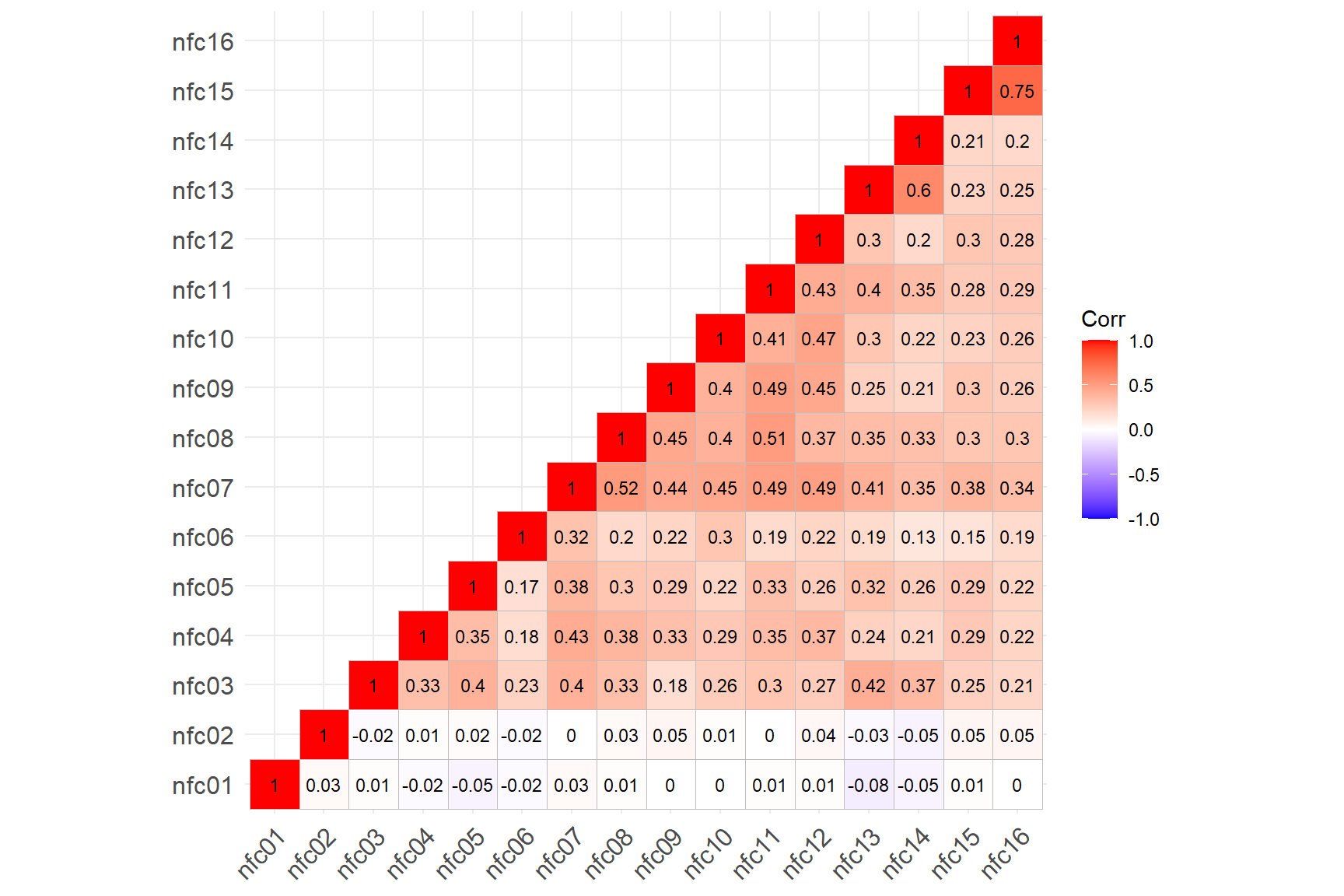
# Now check the internal consistency
reliability_qme <- QME::analyze(test = response_recoded, id = FALSE, na_to_0 = FALSE)

# You can use print(reliability_qme) to view the results.
# If reliability_qme does not print the results, try this:
reliability_qme$test_level
$descriptives
Value
Minimum Score 21.0000000
Maximum Score 112.0000000
Mean Score 80.6228288
Median Score 82.0000000
Standard Deviation 13.1904670
IQR 17.0000000
Skewness (G1) -0.6471103
Kurtosis (G2) 0.7557418
$reliability
Estimate 95% LL 95% UL SEM
Guttman's L2 0.8731550 0.8624677 0.8833207 4.697826
Guttman's L4 0.8932339 0.8842384 0.9017905 4.309996
Feldt-Gilmer 0.8717610 0.8609563 0.8820384 4.723569
Feldt-Brennan 0.8712988 0.8604551 0.8816133 4.732074
Coefficient Alpha 0.8704009 0.8594817 0.8807874 4.748551After replacing the original responses with random values between 1
and 7, we see that the correlation between the first two items and the
remaining items disappeared. In fact, some correlations are even
negative. This finding is not surprising because the randomly-generated
values would not necessarily be correlated with the other items. The
output from the analyze() function shows that the internal
consistency for this new dataset is 0.79 (as opposed to 0.87 in the
original dataset). Given the length of the NFC Scale (16 items), having
two poor quality items significantly decreased the internal consistency
of the scale.
Although this is an exaggerated example, it still demonstrates how to identify problematic items in a given measurement instrument. Using the correlations among the items, discrimination values (i.e., item-total correlation), and the impact of removing each item on the internal consistency, we can identify poor quality items (or potentially problematic items) and shorten our measurement instrument (assuming the remaining items indicate a decent level of internal consistency). There are also more sophisticated ways to identify and remove items for the purpose of creating a shorter instrument, such as the genetic algorithm and ant colony optimization (see my blog post on how to implement these methods in R).
Spearman-Brown prophecy formula
Before we conclude the reliability section, we will also use the
Spearman-Brown prophecy formula to predict the internal consistency of
the NFC Scale depending on the number of items in the instrument. First,
we will examine the scenario where we decide to shorten the length of
the NFC scale by a factor of 0.5 (i.e., reducing the length from 16
items to 8 items). In the earlier analysis, we estimated the internal
consistency of the NFC scale as \(\alpha =
0.87\). Using the spearman.brown() function from
CTT, we will compute how the internal consistency would
change if we reduced the length to 8 items. We specify the current value
of internal consistency (r.xx = 0.87), the desired length
(input = 0.5), and how we want to use the function
(n.or.r = "n" for finding the new internal consistency or
n.or.r = "r" for finding the new length).
$r.new
[1] 0.7699115
The output shows that if we had to reduce the length of the NFC Scale
from 16 items to 8 items, the internal consistency would become roughly
0.77. In the second scenario, we will see how many more items we would
need to increase the internal consistency from 0.87 (current value) to
0.90 (target value). So, we will use input = 0.90 to
indicate our target reliability and n.or.r = "r" to request
for the new length for the NFC scale. We will save the result as n (the
factor that our instrument should be lengthened) and then multiply this
value with the current number of items (16) to find the desired number
of items required for \(\alpha =
0.90\).
# Save the result as n
n <- CTT::spearman.brown(r.xx = 0.87, input = 0.90, n.or.r = "r")

# Multiply it with the current length and round it with zero digits
round(n$n.new * 16, digits = 0)
[1] 22The result above shows that we would need 22 items (i.e., 6 additional items with similar characteristics as the original NFC items) to reach the internal consistency level of 0.90.
Criterion-related validity
In the last step of analyzing the dataset from the NFC Scale, we will examine criterion-related validity. Criterion-related validity indicates how well a measurement instrument predicts the outcome for another instrument measuring the same (or similar construct) construct. If both instruments (i.e., the instrument of interest and the criterion measure) are administered at the same time, we can correlate the scores from the two instruments to check concurrent validity. If we use the scores from the current instrument to predict scores from a criterion measure in the future, then we can obtain evidence for predictive validity.
In the following example, we will calculate the scores for the NFC scale and then correlate the scores with
- self-control scores from the short form of the Self-Control Scale (Bertrams & Dickhäuser, 2009),
- effortful control scores from the Effortful Control Scale of the Adult Temperament Questionnaire (Wiltink et al., 2006), and
- action orientation scores from the Action Control Scale (Kuhl, 1994).
Based on the findings of previous research, we expect to find positive, small to medium associations between NFC and the other three constructs (self-control, effortful control, and action control).
First, we will use the recode() function from the
car package (Fox et al.,
2020) to recode the item scores of 1 to 7 as -3 to +3 for the NFC
Scale and then sum up the item scores to calculate the total score for
the NFC Scale. Since we want to replicate the same recoding procedure
for all 16 items, we will create a custom function for recoding the
items and apply it to the whole dataset using apply(), use
the rowSums() function to calculate the total score for
each person (i.e., the sum of each row in the recoded dataset), obtain a
descriptive summary of the scores using summary(), and
visualize the distribution of the scores using hist().
# Our custom recode function
recode_nfc <- function(x) {
  car::recode(x, "1=-3; 2=-2; 3=-1; 4=0; 5=1; 6=2; 7=3")
}

# Recode the responses
response_recoded <- apply(response_recoded, # data to be modified
                          2, # 2 to apply a function to each column (or 1 for each row)
                          recode_nfc) # Function to be applied


# Compute the NFC Scale scores
nfc_score <- rowSums(response_recoded)

# Summarize the scores
summary(nfc_score)
Min. 1st Qu. Median Mean 3rd Qu. Max.
-43.00 9.00 18.00 16.62 26.00 48.00 # Visualize the distribution of the NFC Scale scores
hist(nfc_score,
xlab = "NFC Scale Score",
main = "Distribution of the NFC Scale Scores")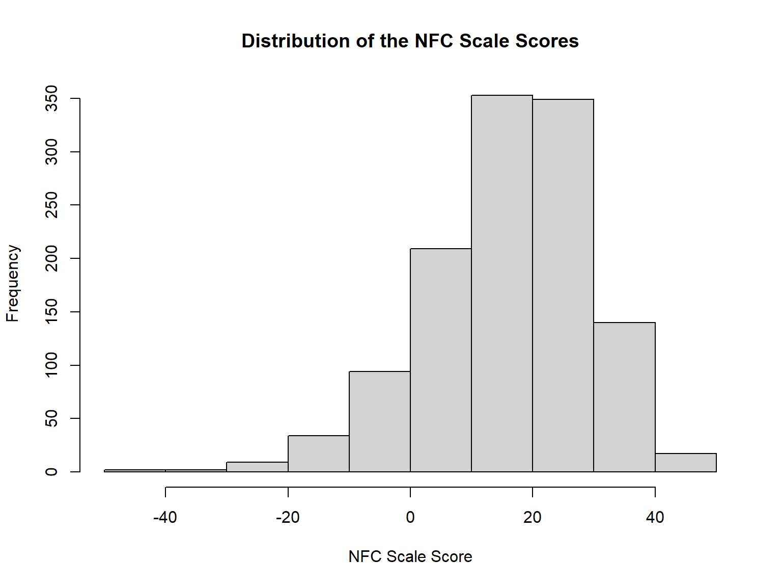
The histogram shows that the NFC Scale scores have a slightly
left-skewed distribution centered around 16.6. Next, we can merge the
scores NFC Scale with the scores from the other scales in a single
dataset. We will use the cbind() function to bind (i.e.,
combine) the four scores. Note that we can use cbind() to
add the columns side by side because we have not
changed the order of respondents in the “response_recoded” and “nfc”
datasets. If we had changed the order of respondents, we would have to
use merge() to merge the datasets based on a common
variable (e.g., the “id” variable) to match the respondents
properly.
Next, we will calculate the correlations among these four scores
(using cor()) and also visualize the correlations (using
ggcorrplot()). cor(), by default, calculates
Pearson correlations between numerical variables. Although we don’t have
any missing scores, we will add
use = "pairwise.complete.obs"–which would keep valid cases
for each pair of variables when calculating the correlations. Without
specifying this option, cor() would fail to calculate the
correlations for a dataset with missing (i.e., NA) values and return
NA.
cormat_scores <- cor(scores, use = "pairwise.complete.obs")

print(cormat_scores)

ggcorrplot::ggcorrplot(corr = cormat_scores,
                       type = "lower",
                       show.diag = TRUE,
                       lab = TRUE,
lab_size = 3) | nfc_score | action_orientation | self_control | effortful_control | |
|---|---|---|---|---|
| nfc_score | 1.00 | 0.28 | 0.26 | 0.29 |
| action_orientation | 0.28 | 1.00 | 0.44 | 0.54 |
| self_control | 0.26 | 0.44 | 1.00 | 0.69 |
| effortful_control | 0.29 | 0.54 | 0.69 | 1.00 |
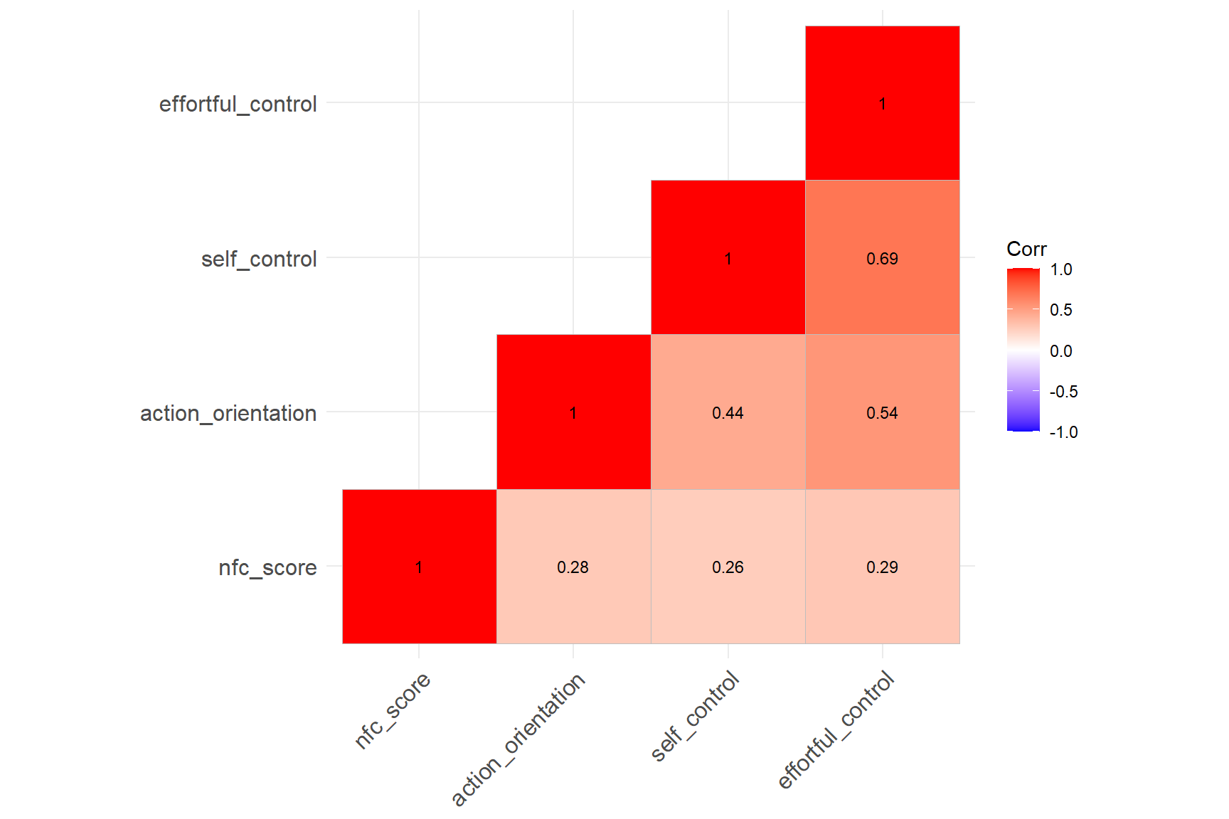
The correlation matrix plot above shows that there is indeed a
positive, small to moderate correlation between the NFC Scale scores and
the scores from the other scales. Remember that these are just raw
correlations among the scale scores. That is, they are
not corrected for attenuation due to the measurement
error involved in each scale. To obtained the disattenuated
correlations, we will use the correct.cor() function from
the psych package. To use this function, we need to
list a raw correlation matrix of scale scores and a vector of
reliability (i.e., internal consistency) estimates. The reliability
estimate for the NFC Scale is 0.87 and the reliability estimates for the
three criterion measures are (Grass et al.,
2019):
- The Action Control Scale: 0.791
- The Self-Control Scale: 0.817
- The Effortful Control Scale: 0.783
Using this information, we can calculate the disattenuated correlations as follows:
psych::correct.cor(x = cormat_scores, # Raw correlation matrix
y = c(0.87, 0.791, 0.817, 0.783)) # Reliability values in the same order as cormat_scores| nfc_score | action_orientation | self_control | effortful_control | |
|---|---|---|---|---|
| nfc_score | 0.87 | 0.34 | 0.31 | 0.35 |
| action_orientation | 0.28 | 0.79 | 0.54 | 0.69 |
| self_control | 0.26 | 0.44 | 0.82 | 0.87 |
| effortful_control | 0.29 | 0.54 | 0.69 | 0.78 |
In the new correlation matrix above, the upper-diagonal part shows the correlations among the four scale scores that have been corrected for attenuation, the diagonal part shows the reliability estimates for the four scales, and the lower-diagonal part shows the original (i.e., raw) correlations among the four scale scores. After applying the correction for attenuation, the new correlation values have become higher than their raw counterparts. For example, the scores from the NFC scale has a correlation of \(r = .29\) with the scores from the Effortful Control Scale, whereas the corrected correlation between the two scales is \(r = .35\).
In addition to the relationship between the total scores from the NFC
Scale and the criterion measures, we can also calculate item-validity
index (IVI) to check the relationship between each item in the NFC Scale
and the scores from the criterion measures. IVI can range between -0.5
and 0.5, with large values (in absolute magnitude) indicative of higher
validity. In the following example, we will create a custom IVI function
and apply it to the NFC Scale to calculate the IVI values using the
action orientation scores as a criterion measure (the ivi()
function originally comes from the hemp
package).
# Custom function for calculating item-validity index
ivi <- function(item, criterion) {
    s_i <- sd(item, na.rm = TRUE)
    r <- cor(item, criterion, use = "complete.obs")
    index <- s_i * r
    return(index)
}

# Apply the ivi function to the NFC items
nfc_ivi <- apply(response_recoded,
                 2,
                 function(x) ivi(item = x, criterion = nfc$action_orientation))

# Save the results as a data frame and print them
nfc_ivi <- as.data.frame(nfc_ivi)
print(nfc_ivi)
nfc_ivi
nfc01 0.37297915
nfc02 0.21153487
nfc03 0.19981987
nfc04 0.14540417
nfc05 0.06209198
nfc06 0.20228579
nfc07 0.26048244
nfc08 0.25950684
nfc09 0.25584111
nfc10 0.44981819
nfc11 0.27994998
nfc12 0.24413937
nfc13 0.29590845
nfc14 0.29309729
nfc15 0.03979380
nfc16 0.10474004The output above shows that most items in the NFC Scale have small to moderate correlations with the action orientation scores (just like the total scores from the NFC Scale), except for nfc05 and nfc15. This finding provides additional evidence supporting the validity of the NFC Scale.
Example 2: A Multiple-Choice Exam
In addition to ordinal response data from psychological instruments,
we also use CTT to analyze dichotomous (i.e., binary) response data from
educational instruments (e.g., multiple-choice exams). With dichotomous
response data, we can conduct not only the CTT-based analyses we have
have demonstrated above but also additional analyses specific to
educational assessments, such as distractor analysis. In the following
example, we will use a dataset that consists of the responses of 651
university students to the Homeostasis Concept Inventory (HCI)
multiple-choice test. This dataset originally comes from the
ShinyItemAnalysis package (see
?ShinyItemAnalysis::HCItest). A clean version of the
dataset as a comma-separated-values file (hci.csv) is available here. The file has
the following variables:
- item1 to item20: Answers to multiple-choice items (A, B, C, D, or E)
- gender: “F” for female and “M” for male
- eng_first_lang: “yes” if English is the student’s first language, otherwise “no”
- study_year: The student’s year of study at the university
- major: 1 if the student plans to major in the life sciences, otherwise 0
Setting up R
We will begin our analysis by importing the hci.csv dataset into R. Then we will
print the first six rows using the head() function and the
structure of the dataset using the str() function:
# Import the dataset
hci <- read.csv("hci.csv", header = TRUE)

# Print the first 6 rows of the dataset
# You can use head(hci, 10) to print the first 10 rows instead of 6 (default)
head(hci)

# See the structure of the dataset
str(hci)
item1 item2 item3 item4 item5 item6 item7 item8 item9 item10 item11 item12 item13 item14 item15 item16
1 D B A D B B B C D A A D A A D A
2 D B A D B C B C D A A D A A C A
3 D B A D C C B C D A A D A A A A
4 D B A D B C C C D A A D A A C A
5 D B A D B C C C D A A D A A D A
6 D B A D B C C C D A A D A A C A
item17 item18 item19 item20 gender eng_first_lang study_year major
1 D C C D F yes 4 1
2 C C C D F yes 4 1
3 C C C D M yes 4 1
4 C C C D M yes 4 1
5 C C C D M yes 4 1
6 C C C D F yes 4 1'data.frame': 651 obs. of 24 variables:
$ item1 : chr "D" "D" "D" "D" ...
$ item2 : chr "B" "B" "B" "B" ...
$ item3 : chr "A" "A" "A" "A" ...
$ item4 : chr "D" "D" "D" "D" ...
$ item5 : chr "B" "B" "C" "B" ...
$ item6 : chr "B" "C" "C" "C" ...
$ item7 : chr "B" "B" "B" "C" ...
$ item8 : chr "C" "C" "C" "C" ...
$ item9 : chr "D" "D" "D" "D" ...
$ item10 : chr "A" "A" "A" "A" ...
$ item11 : chr "A" "A" "A" "A" ...
$ item12 : chr "D" "D" "D" "D" ...
$ item13 : chr "A" "A" "A" "A" ...
$ item14 : chr "A" "A" "A" "A" ...
$ item15 : chr "D" "C" "A" "C" ...
$ item16 : chr "A" "A" "A" "A" ...
$ item17 : chr "D" "C" "C" "C" ...
$ item18 : chr "C" "C" "C" "C" ...
$ item19 : chr "C" "C" "C" "C" ...
$ item20 : chr "D" "D" "D" "D" ...
$ gender : chr "F" "F" "M" "M" ...
$ eng_first_lang: chr "yes" "yes" "yes" "yes" ...
$ study_year : int 4 4 4 4 4 4 4 4 4 3 ...
$ major : int 1 1 1 1 1 1 1 1 1 1 ...Except for “study_year”, all the other variables in our dataset are
categorical (note that despite being an integer, “major” is also a
categorical variable identifying the student’s plan to major in the life
sciences where 1 means yes and 0 means no). Given that almost all the
variables are categorical, we can use plot_bar() from
DataExplorer to visualize the variables. We will use
nrow = 6, ncol = 4 arguments to print the bar plots in a 6
x 4 layout.
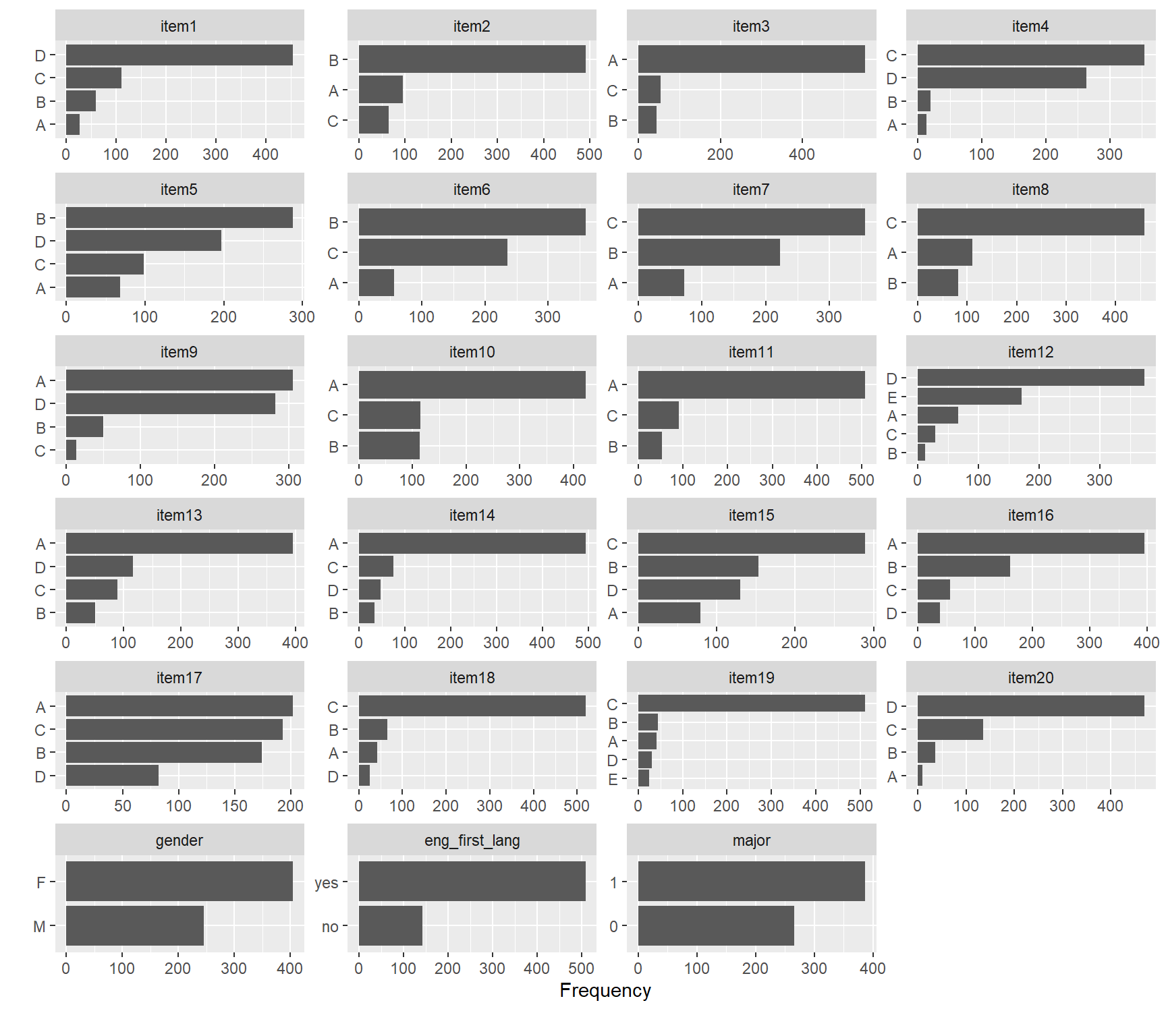
The bar plots above show the distribution of response options for
each item and the number of categories for each categorical variables
(gender, English as the first language, and major). The
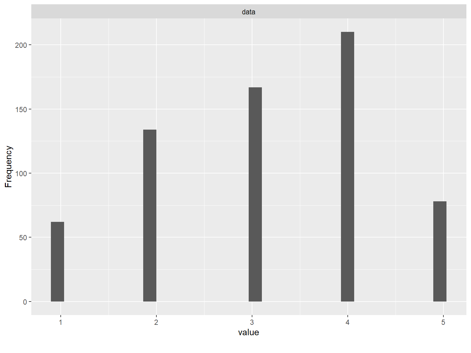
plot_bar() function skipped the variable “study_year” since
it is a continuous variable (although it is a continuous variable with a
limited range of 1 to 5). We can plot “study_year” using
plot_histogram().
Distractor analysis
Multiple-choice items typically consist of a correct response option (i.e., keyed option) and a bunch of incorrect response options known as “distractors”. When answering the items, students who know the content adequately are expected to select the keyed option whereas students who have little to no knowledge of the content are expected to select one of the distractors. A distractor may be implausible due to several reasons such as:
- mostly students with adequate content knowledge select the distractor
- almost no student selects the distractor
- most students (including those with adequate content knowledge) selects the distractor over the keyed option
To identify such cases and determine whether the distractors are
plausible, we conduct distractor analysis. Distractor analysis refers to
the analysis of response options of multiple-choice items in terms of
their frequency (or proportions). In the following example, we will use
the hci dataset and conduct distractor analysis using different
packages. To run distractor analysis, we need the response data (with
response options of A, B, C, D etc.) and the answer key for the items.
The answer key for the hci dataset is available here (also see
?ShinyItemAnalysis::HCIkey). So, we will import the answer
key into R:
# Import the answer key
key <- read.csv("hci_key.csv", header = TRUE)

# Print the answer key
print(key)
key
1 D
2 B
3 A
4 D
5 B
6 C
7 C
8 C
9 D
10 A
11 A
12 D
13 A
14 A
15 C
16 A
17 C
18 C
19 C
20 DNow we will select only the items in the hci dataset and then conduct distractor analysis. Since all the items in the dataset start with “item”, we can use this word to select the items very easily:
hci_items <- dplyr::select(hci, # name of the dataset
                           starts_with("item")) # variables to be selected

head(hci_items)
item1 item2 item3 item4 item5 item6 item7 item8 item9 item10 item11 item12 item13 item14 item15 item16
1 D B A D B B B C D A A D A A D A
2 D B A D B C B C D A A D A A C A
3 D B A D C C B C D A A D A A A A
4 D B A D B C C C D A A D A A C A
5 D B A D B C C C D A A D A A D A
6 D B A D B C C C D A A D A A C A
item17 item18 item19 item20
1 D C C D
2 C C C D
3 C C C D
4 C C C D
5 C C C D
6 C C C DNext, we will use distractorAnalysis() from the
CTT package to conduct distractor analysis:
$item1
  correct key   n       rspP       pBis     discrim      lower      mid50       mid75      upper
A           A  27 0.04147465 -0.2461507 -0.09049774 0.09049774 0.05263158 0.005524862 0.00000000
B           B  59 0.09062980 -0.1662783 -0.05838780 0.11764706 0.07017544 0.093922652 0.05925926
C           C 110 0.16897081 -0.4081448 -0.28422993 0.32126697 0.16666667 0.082872928 0.03703704
D       *   D 455 0.69892473  0.2884191  0.43311547 0.47058824 0.71052632 0.817679558 0.90370370
E           E   0 0.00000000         NA  0.00000000 0.00000000 0.00000000 0.000000000 0.00000000

$item2
  correct key   n       rspP       pBis     discrim     lower     mid50      mid75      upper
A           A  96 0.14746544 -0.3951782 -0.24062343 0.2850679 0.1140351 0.07734807 0.04444444
B       *   B 490 0.75268817  0.2206134  0.32575834 0.5927602 0.7280702 0.83977901 0.91851852
C           C  65 0.09984639 -0.1896673 -0.08513491 0.1221719 0.1578947 0.08287293 0.03703704
D           D   0 0.00000000         NA  0.00000000 0.0000000 0.0000000 0.00000000 0.00000000
E           E   0 0.00000000         NA  0.00000000 0.0000000 0.0000000 0.00000000 0.00000000

$item3
  correct key   n       rspP       pBis    discrim     lower      mid50      mid75       upper
A       *   A 552 0.84792627  0.3500418  0.3229093 0.6696833 0.82456140 0.97237569 0.992592593
B           B  45 0.06912442 -0.3794204 -0.1583710 0.1583710 0.07017544 0.01104972 0.000000000
C           C  54 0.08294931 -0.3411496 -0.1645383 0.1719457 0.10526316 0.01657459 0.007407407
D           D   0 0.00000000         NA  0.0000000 0.0000000 0.00000000 0.00000000 0.000000000
E           E   0 0.00000000         NA  0.0000000 0.0000000 0.00000000 0.00000000 0.000000000

$item4
  correct key   n       rspP       pBis     discrim      lower      mid50       mid75     upper
A           A  14 0.02150538 -0.2471775 -0.05882353 0.05882353 0.00877193 0.000000000 0.0000000
B           B  20 0.03072197 -0.2652578 -0.08144796 0.08144796 0.00877193 0.005524862 0.0000000
C           C 354 0.54377880 -0.2883596 -0.28493380 0.61085973 0.59649123 0.591160221 0.3259259
D       *   D 263 0.40399386  0.1729866  0.42520530 0.24886878 0.38596491 0.403314917 0.6740741
E           E   0 0.00000000         NA  0.00000000 0.00000000 0.00000000 0.000000000 0.0000000

$item5
  correct key   n      rspP       pBis    discrim     lower     mid50      mid75      upper
A           A  68 0.1044547 -0.2274639 -0.1122842 0.1493213 0.1228070 0.08839779 0.03703704
B       *   B 288 0.4423963  0.2767838  0.5297134 0.2036199 0.4649123 0.50276243 0.73333333
C           C  98 0.1505376 -0.2614192 -0.1118485 0.2081448 0.1578947 0.11602210 0.09629630
D           D 197 0.3026114 -0.3195977 -0.3055807 0.4389140 0.2543860 0.29281768 0.13333333
E           E   0 0.0000000         NA  0.0000000 0.0000000 0.0000000 0.00000000 0.00000000

$item6
  correct key   n       rspP       pBis    discrim     lower     mid50      mid75       upper
A           A  56 0.08602151 -0.3026338 -0.1464387 0.1538462 0.1315789 0.03314917 0.007407407
B           B 359 0.55145929 -0.4253397 -0.4054634 0.7239819 0.6228070 0.46961326 0.318518519
C       *   C 236 0.36251920  0.3418847  0.5519021 0.1221719 0.2456140 0.49723757 0.674074074
D           D   0 0.00000000         NA  0.0000000 0.0000000 0.0000000 0.00000000 0.000000000
E           E   0 0.00000000         NA  0.0000000 0.0000000 0.0000000 0.00000000 0.000000000

$item7
  correct key   n      rspP       pBis    discrim     lower     mid50     mid75      upper
A           A  72 0.1105991 -0.2413236 -0.1242165 0.1538462 0.1140351 0.1160221 0.02962963
B           B 223 0.3425499 -0.2651716 -0.1582705 0.4027149 0.3947368 0.3093923 0.24444444
C       *   C 356 0.5468510  0.1009380  0.2824870 0.4434389 0.4912281 0.5745856 0.72592593
D           D   0 0.0000000         NA  0.0000000 0.0000000 0.0000000 0.0000000 0.00000000
E           E   0 0.0000000         NA  0.0000000 0.0000000 0.0000000 0.0000000 0.00000000

$item8
  correct key   n      rspP       pBis    discrim     lower     mid50      mid75      upper
A           A 110 0.1689708 -0.3799236 -0.2871125 0.3167421 0.1666667 0.09392265 0.02962963
B           B  82 0.1259601 -0.3515895 -0.1994972 0.2217195 0.1403509 0.07734807 0.02222222
C       *   C 459 0.7050691  0.3252153  0.4866097 0.4615385 0.6929825 0.82872928 0.94814815
D           D   0 0.0000000         NA  0.0000000 0.0000000 0.0000000 0.00000000 0.00000000
E           E   0 0.0000000         NA  0.0000000 0.0000000 0.0000000 0.00000000 0.00000000

$item9
  correct key   n       rspP       pBis     discrim      lower      mid50      mid75      upper
A           A 306 0.47004608 -0.3031336 -0.30718954 0.52941176 0.52631579 0.54696133 0.22222222
B           B  50 0.07680492 -0.2709100 -0.09582705 0.14027149 0.05263158 0.03867403 0.04444444
C           C  13 0.01996928 -0.2320653 -0.05882353 0.05882353 0.00000000 0.00000000 0.00000000
D       *   D 282 0.43317972  0.2129679  0.46184012 0.27149321 0.42105263 0.41436464 0.73333333
E           E   0 0.00000000         NA  0.00000000 0.00000000 0.00000000 0.00000000 0.00000000

$item10
  correct key   n      rspP       pBis    discrim     lower     mid50     mid75      upper
A       *   A 422 0.6482335  0.2643568  0.4915368 0.4343891 0.5701754 0.7513812 0.92592593
B           B 114 0.1751152 -0.3273501 -0.2463885 0.2760181 0.2017544 0.1436464 0.02962963
C           C 115 0.1766513 -0.3437457 -0.2451483 0.2895928 0.2280702 0.1049724 0.04444444
D           D   0 0.0000000         NA  0.0000000 0.0000000 0.0000000 0.0000000 0.00000000
E           E   0 0.0000000         NA  0.0000000 0.0000000 0.0000000 0.0000000 0.00000000

$item11
  correct key   n       rspP       pBis    discrim     lower      mid50      mid75      upper
A       *   A 507 0.77880184  0.2851116  0.3582705 0.5972851 0.75438596 0.88397790 0.95555556
B           B  53 0.08141321 -0.3704061 -0.1764706 0.1764706 0.07017544 0.03314917 0.00000000
C           C  91 0.13978495 -0.3118272 -0.1817999 0.2262443 0.17543860 0.08287293 0.04444444
D           D   0 0.00000000         NA  0.0000000 0.0000000 0.00000000 0.00000000 0.00000000
E           E   0 0.00000000         NA  0.0000000 0.0000000 0.00000000 0.00000000 0.00000000

$item12
  correct key   n       rspP       pBis     discrim      lower      mid50      mid75      upper
A           A  66 0.10138249 -0.2708640 -0.14067371 0.16289593 0.13157895 0.06629834 0.02222222
B           B  12 0.01843318 -0.1478828 -0.01685939 0.03167421 0.00877193 0.01104972 0.01481481
C           C  29 0.04454685 -0.2144364 -0.07239819 0.07239819 0.06140351 0.03314917 0.00000000
D       *   D 373 0.57296467  0.3155934  0.53759008 0.34389140 0.48245614 0.67955801 0.88148148
E           E 171 0.26267281 -0.3558190 -0.30765879 0.38914027 0.31578947 0.20994475 0.08148148

$item13
  correct key   n       rspP       pBis    discrim     lower     mid50      mid75       upper
A       *   A 396 0.60829493  0.3612177  0.5877996 0.3529412 0.4473684 0.77348066 0.940740741
B           B  50 0.07680492 -0.2922788 -0.1373890 0.1447964 0.0877193 0.03867403 0.007407407
C           C  89 0.13671275 -0.3357834 -0.2056645 0.2352941 0.1929825 0.06077348 0.029629630
D           D 116 0.17818740 -0.3207030 -0.2447461 0.2669683 0.2719298 0.12707182 0.022222222
E           E   0 0.00000000         NA  0.0000000 0.0000000 0.0000000 0.00000000 0.000000000

$item14
  correct key   n       rspP       pBis     discrim      lower      mid50      mid75      upper
A       *   A 494 0.75883257  0.3385578  0.43807609 0.52488688 0.74561404 0.90055249 0.96296296
B           B  34 0.05222734 -0.2222059 -0.07115804 0.08597285 0.09649123 0.01104972 0.01481481
C           C  76 0.11674347 -0.3161656 -0.19949723 0.22171946 0.11403509 0.06077348 0.02222222
D           D  47 0.07219662 -0.3581467 -0.16742081 0.16742081 0.04385965 0.02762431 0.00000000
E           E   0 0.00000000         NA  0.00000000 0.00000000 0.00000000 0.00000000 0.00000000

$item15
  correct key   n      rspP       pBis     discrim     lower     mid50     mid75      upper
A           A  79 0.1213518 -0.2416434 -0.12213843 0.2036199 0.0877193 0.0718232 0.08148148
B           B 153 0.2350230 -0.4241449 -0.34757835 0.3846154 0.3245614 0.1436464 0.03703704
C       *   C 289 0.4439324  0.3005640  0.56346573 0.2217195 0.3333333 0.5303867 0.78518519
D           D 130 0.1996928 -0.1593722 -0.09374895 0.1900452 0.2543860 0.2541436 0.09629630
E           E   0 0.0000000         NA  0.00000000 0.0000000 0.0000000 0.0000000 0.00000000

$item16
  correct key   n       rspP       pBis     discrim      lower      mid50      mid75      upper
A       *   A 395 0.60675883  0.3822268  0.58079437 0.33031674 0.55263158 0.75138122 0.91111111
B           B 161 0.24731183 -0.4452814 -0.38089492 0.42533937 0.28947368 0.15469613 0.04444444
C           C  56 0.08602151 -0.3213548 -0.15260600 0.16742081 0.08771930 0.03867403 0.01481481
D           D  39 0.05990783 -0.1517499 -0.04729345 0.07692308 0.07017544 0.05524862 0.02962963
E           E   0 0.00000000         NA  0.00000000 0.00000000 0.00000000 0.00000000 0.00000000

$item17
  correct key   n      rspP        pBis     discrim     lower     mid50     mid75      upper
A           A 202 0.3102919 -0.09020780  0.02808782 0.2533937 0.3684211 0.3646409 0.28148148
B           B 174 0.2672811 -0.29346777 -0.22289258 0.3710407 0.1929825 0.2762431 0.14814815
C       *   C 193 0.2964670  0.04340407  0.24290263 0.2533937 0.2456140 0.2320442 0.49629630
D           D  82 0.1259601 -0.13266468 -0.04809787 0.1221719 0.1929825 0.1270718 0.07407407
E           E   0 0.0000000          NA  0.00000000 0.0000000 0.0000000 0.0000000 0.00000000

$item18
  correct key   n       rspP       pBis     discrim      lower      mid50      mid75       upper
A           A  42 0.06451613 -0.3140941 -0.12833920 0.13574661 0.05263158 0.02762431 0.007407407
B           B  65 0.09984639 -0.4090210 -0.21307190 0.23529412 0.07017544 0.01104972 0.022222222
C       *   C 519 0.79723502  0.4171207  0.42738395 0.54298643 0.84210526 0.95027624 0.970370370
D           D  25 0.03840246 -0.2569481 -0.08597285 0.08597285 0.03508772 0.01104972 0.000000000
E           E   0 0.00000000         NA  0.00000000 0.00000000 0.00000000 0.00000000 0.000000000

$item19
  correct key   n       rspP       pBis     discrim      lower      mid50      mid75       upper
A           A  41 0.06298003 -0.2840018 -0.11023965 0.11764706 0.07017544 0.03314917 0.007407407
B           B  44 0.06758833 -0.3302629 -0.13450645 0.14932127 0.05263158 0.01657459 0.014814815
C       *   C 511 0.78494624  0.3665060  0.41833417 0.55203620 0.80701754 0.91712707 0.970370370
D           D  30 0.04608295 -0.2013994 -0.07856544 0.08597285 0.05263158 0.02209945 0.007407407
E           E  25 0.03840246 -0.2483756 -0.09502262 0.09502262 0.01754386 0.01104972 0.000000000

$item20
  correct key   n       rspP       pBis     discrim      lower      mid50      mid75      upper
A           A  10 0.01536098 -0.1639141 -0.04072398 0.04072398 0.00877193 0.00000000 0.00000000
B           B  36 0.05529954 -0.3382951 -0.13574661 0.13574661 0.02631579 0.01657459 0.00000000
C           C 135 0.20737327 -0.3909296 -0.28915703 0.34841629 0.21929825 0.13812155 0.05925926
D       *   D 470 0.72196621  0.3395533  0.46562762 0.47511312 0.74561404 0.84530387 0.94074074
E           E   0 0.00000000         NA  0.00000000 0.00000000 0.00000000 0.00000000 0.00000000
In the output, we see the keyed option for each item (shown with *), the number of students who selected each response option (n), the proportion of students who selected each response option (rspP), point-biserial correlation between the response option and the total score with the item removed (pBis), discrimination of the response option calculated as the upper proportion minus the lower proportion (discrim), proportion of students from the lowest score group choosing the response option (lower), and proportion of students from the highest score group choosing the response option (higher). We expect most students from the mid75 and upper groups to choose the keyed option. For example, in item 1, nearly 70% of the students selected the keyed option of D. We see that the proportion of students answering the item correctly is increasing as we move from the lower group (43%) to the upper group (90%). The opposite trend seems to occur for the distractors (i.e., A, B, and C).
We can also go over the items one by one and identify if there are any items where distractors did not seem to attract enough students. For example, in item 20, two distractors (A and B) were only selected by 1.5% and 5.5% of the students, respectively. Most students either selected the keyed option of D or option C as one of the distractors. The distractors of this particular item should be examined to increase the plausibility of the first two distractors. A similar issue is happening with item 18 where only 3.8% of the students selected option D and item 12 where only 1.8% of the students selected option B. We also see that for all of the items, the distractors have negative pBis and discrim values whereas the keyed options have positive values for the same indices, suggesting that the items function properly.
distractorAnalysis() calculates the total score for each
student by comparing the responses to the answer key and uses the total
score to split students into four groups (lower, mid50, mid75, upper).
If we wanted to increase or decrease the number of groups, we could use
the nGroups argument in distractorAnalysis()
(e.g., nGroups = 6 to run the analysis with 6 groups based
on the total score). Alternatively, we could use the
defineGroups argument to define the quantile breakpoints
for groups based on the total score (e.g.,
defineGroups = c(.25,.50,.25) to request three groups with
25% of the students in the top and the bottom groups and the remaining
50% in the middle group). In addition, we can save the distractor
analysis results into a comma-separated-values (csv) file by using the
csvReport argument in distractorAnalysis()
(e.g., csvReport = "hci_distactors.csv")
In addition to distractorAnalysis() from the
CTT package, we can also use the analyze()
from the QME package to conduct distractor analysis and
obtain nice visualizations of each item and its response options. The
QME package requires the answer key to be set up in a
certain way (either a vector or a full data frame). In the hci dataset,
some items have only three response options (A, B, or C), whereas the
others have 4 (A, B, C, or D) or 5 (A, B, C, D, and E) response options.
For this type of dataset, the data frame answer key is the ideal option.
You can find the reconfigured answer key for the hci dataset here. We will
import the new answer key into R, conduct item analysis using
analyze(), and use the outcome of this analysis in
distractor_report() to obtain a distractor report for the
hci items.
# Import the new answer key
key2 <- read.csv("hci_key2.csv" , header = TRUE)

# View the new answer key
print(key2)

# Conduct analysis with analyze() and save the results
hci_analysis <- QME::analyze(test = hci_items, key = key2, id = FALSE)

# Create a distractor report
QME::distractor_report(x = hci_analysis)
The report returned from distractor_report() is quite
long. So, we will only have a look at the output from a sample item
(item 1) below.
### Details for `item1`


|Choice | Key| Proportions| Response Discrimination|
|:------|---:|-----------:|-----------------------:|
|A      |   0|        0.04|                   -0.23|
|B      |   0|        0.09|                   -0.09|
|C      |   0|        0.17|                   -0.29|
|D      |   1|        0.70|                    0.29|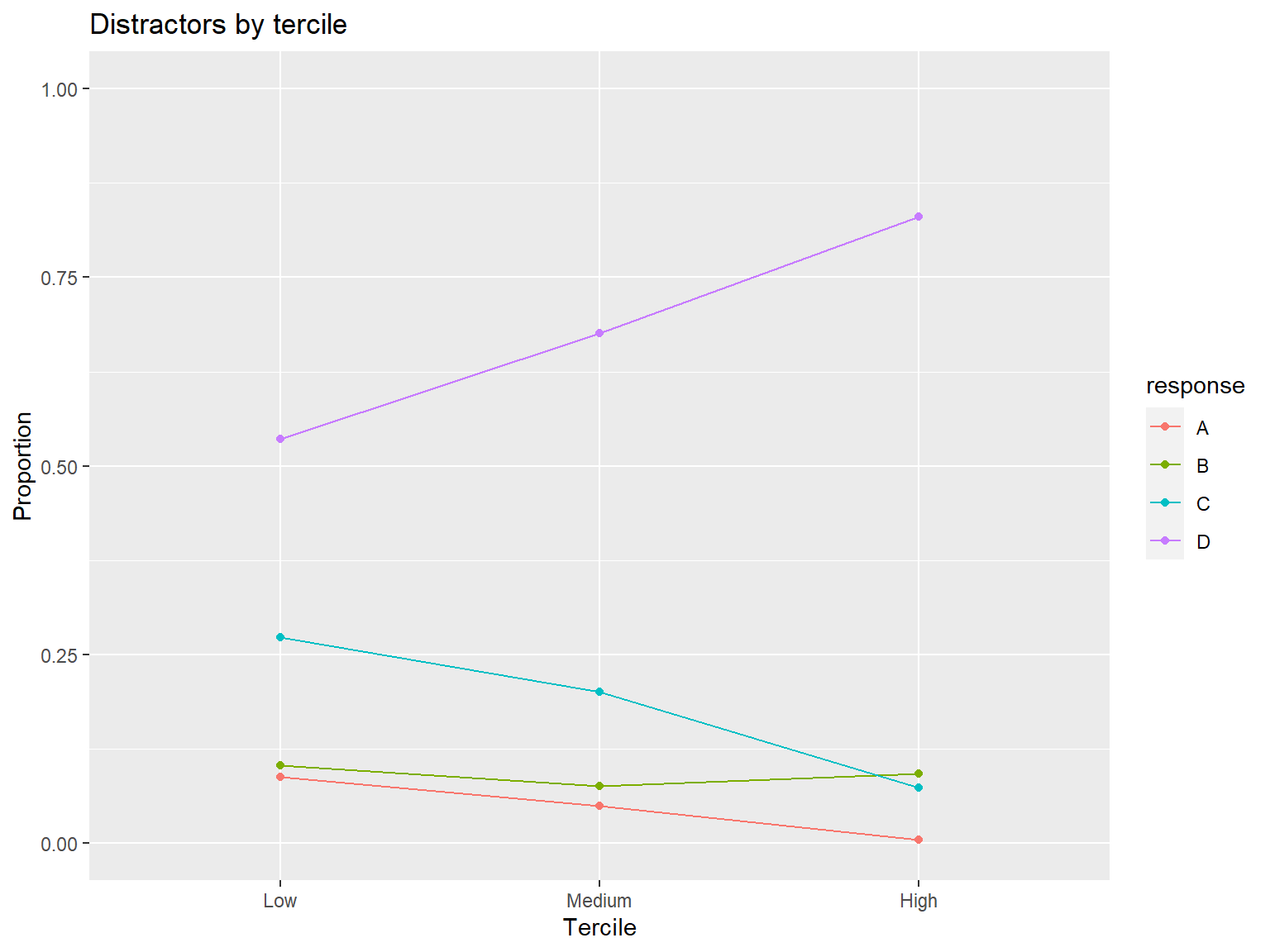
The table shows us the the response options (choice), the answer key (where it is “1”), proportions of students selecting each response option (proportions), and discrimination values for the response options (response discrimination). We also see similar results in the figure above but the proportions of students for each response option are split into three groups (i.e., tercile): low, medium, and high. Tercile refers to three groups where each contains a third of the total sample. The figure shows that as we move from the low to high group, the proportions of students selecting the keyed answer (D) is increasing, whereas the proportions of students selecting the distractors (A, B, or C) are decreasing. This finding suggests that the response options of item 1 function as expected.
Lastly, if we are interested in creating a distractor functioning
figure (similar to the one from the QME package) for a
specific item, plotDistractorAnalysis() from the
ShinyItemAnalysis package is a better option due to its
ease of use. To use this function, we will save the answer key as a
vector (called “key3” this time). The function uses the raw responses
(Data = hci_items), the answer key
(key = key3), the number of groups to create based on the
total score (num.groups = 3), and the item to be plotted
(item = 1). There are also additional arguments to
customize the function, such as criterion to specify an
external score variable instead of calculating the total score and
cut.points to specify what cut-off points should be used to
create the groups according to num.groups (see
?ShinyItemAnalysis::plotDistractorAnalysis for further
details).
# Save the key column from the key data frame as a vector
key3 <- as.vector(key$key)

ShinyItemAnalysis::plotDistractorAnalysis(Data = hci_items, # response data to be analyzed
                                          key = key3, # answer key
                                          num.groups = 3, # how many student groups we want (default is 3)
                                          item = 1) # the number of the item to be plotted
$item1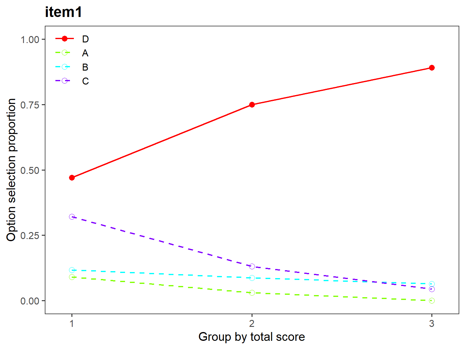
The plot returned from plotDistractorAnalysis() is very
similar to the one from distractor_report() although they
are not necessarily identical due to the way student groups are created
by the QME and ShinyItemAnalysis
packages.
Scoring and scaling
To conduct further analysis with the items in the hci dataset, we
need to transform raw responses (i.e., A, B, C, D, and E) to item scores
(i.e., 1 for correct and 0 for incorrect). This procedure is called
“scoring”. To score the items the hci datasets, we could write a custom
scoring function that compares the responses to a given item to the
answer key and scores the item dichotomously (i.e., 1 or 0). Then, we
would have to apply this function to the entire dataset using a loop
(i.e., repeating the process across items and/or students). Luckily, the
CTT package already includes a score()
function that calculates item scores, finds the sum of the item scores
(i.e., total scores), and computes coefficient alpha in a single
analysis. The score() function requires the answer key to
be a vector instead of a data frame. So, we will first save the answer
key as a vector (called “key3” this time) and then score the items using
the answer key.
# Score the items
hci_scored <- CTT::score(items = hci_items, # data to be scored
                         key = key3, # answer key
                         output.scored = TRUE, # save the scored items
                         rel = TRUE) # calculate reliability for the scored items

# Now let's see what's in hci_scored
str(hci_scored)
List of 3
$ score : Named num [1:651] 16 19 17 20 19 20 20 14 18 17 ...
..- attr(*, "names")= chr [1:651] "P1" "P2" "P3" "P4" ...
$ reliability:List of 9
..$ nItem : int 20
..$ nPerson : int 651
..$ alpha : num 0.715
..$ scaleMean : num 12.2
..$ scaleSD : num 3.64
..$ alphaIfDeleted: num [1:20(1d)] 0.704 0.71 0.701 0.715 0.705 ...
..$ pBis : num [1:20(1d)] 0.288 0.221 0.35 0.173 0.277 ...
..$ bis : num [1:20(1d)] 0.37 0.295 0.525 0.218 0.344 ...
..$ itemMean : Named num [1:20] 0.699 0.753 0.848 0.404 0.442 ...
.. ..- attr(*, "names")= chr [1:20] "item1" "item2" "item3" "item4" ...
..- attr(*, "class")= chr "reliability"
$ scored : num [1:651, 1:20] 1 1 1 1 1 1 1 0 1 1 ...
..- attr(*, "dimnames")=List of 2
.. ..$ : NULL
.. ..$ : chr [1:20] "item1" "item2" "item3" "item4" ...The structure of hci_scored shows that we have three
sets of information in this object:
scoreshows the total scores of the students based on the scored itemsreliabilityshows the internal consistency of the scored hci itemsscoredshows the scored hci items
Now, let’s take a look at each part one by one. First, we will begin with the total scores. We will save the scores as a separate dataset and then analyze it descriptively and visually.
# Save the scores as a separate variable
scores <- hci_scored$score

# Summarize the scores
summary(scores)
Min. 1st Qu. Median Mean 3rd Qu. Max.
3.00 10.00 12.00 12.21 15.00 20.00 # Visualize the distribution of the scores using a histogram
# We will also customize the histogram a little bit
hist(x = scores, # scores to be visualized
xlab = "Total Score", # label for the x axis
main = "Distribution of HCI Total Scores", # title for the plot
col = "lightblue", # colour for the bars in the histogram
breaks = 15, # number of breakpoints for the histogram
xlim = c(0, 20)) # minimum and maximum values for the x axis
# Add a red, vertical line showing the mean
abline(v = mean(scores), col = "red", lwd = 2, lty = 2)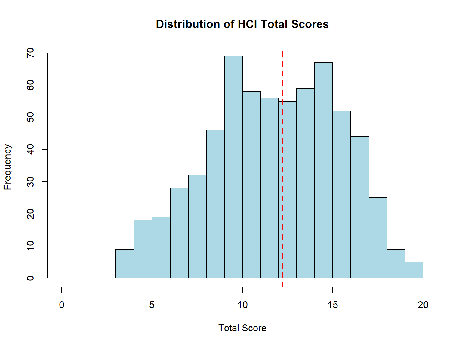
Second, we will check out the reliability information.
 Number of Items
 20

 Number of Examinees
 651

 Coefficient Alpha
 0.715
Lastly, we will see the scored versions of the items in the hci dataset:
# Save the scored items
hci_items_scored <- hci_scored$scored

# Print the first six rows of this dataset
head(hci_items_scored)
item1 item2 item3 item4 item5 item6 item7 item8 item9 item10 item11 item12 item13 item14 item15 item16
[1,] 1 1 1 1 1 0 0 1 1 1 1 1 1 1 0 1
[2,] 1 1 1 1 1 1 0 1 1 1 1 1 1 1 1 1
[3,] 1 1 1 1 0 1 0 1 1 1 1 1 1 1 0 1
[4,] 1 1 1 1 1 1 1 1 1 1 1 1 1 1 1 1
[5,] 1 1 1 1 1 1 1 1 1 1 1 1 1 1 0 1
[6,] 1 1 1 1 1 1 1 1 1 1 1 1 1 1 1 1
item17 item18 item19 item20
[1,] 0 1 1 1
[2,] 1 1 1 1
[3,] 1 1 1 1
[4,] 1 1 1 1
[5,] 1 1 1 1
[6,] 1 1 1 1Assume that we want to rescale the total scores (out of 20) to have a
mean of 50 and standard deviation of 10 (just like T-scores). To
accomplish such transformation, we can use
score.transform() from the CTT package. In
the following example, we will rescale the total scores from the hci
dataset and then draw a histogram of the scaled scores.
scores_scaled <- CTT::score.transform(scores = scores, # scores to be rescaled
                                      mu.new = 50, # mean of the new scale
                                      sd.new = 15) # standard deviation of the new scale


# Visualize the distribution of the scaled scores using a histogram
hist(x = scores_scaled$new.scores,
     xlab = "Scaled Score",
     main = "Distribution of HCI Scaled Scores",
     col = "lightblue",
     xlim = c(0, 100))

# Add a red, vertical line showing the mean
abline(v = mean(scores_scaled$new.scores), col = "red", lwd = 2, lty = 2)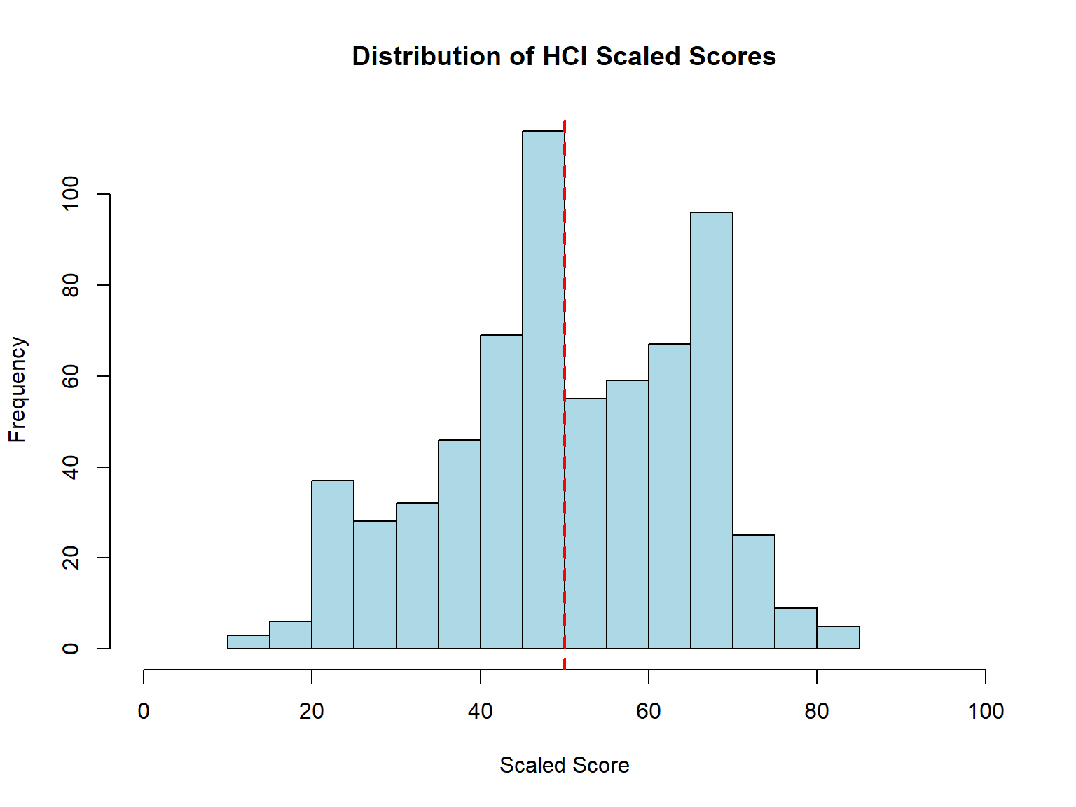
We can also force the scores to follow a normal distribution using
the normalize argument:
scores_scaled2 <- CTT::score.transform(scores = scores, # scores to be rescaled
                                       mu.new = 50, # mean of the new scale
                                       sd.new = 15, # standard deviation of the new scale
                                       normalize = TRUE) # If TRUE, normalize the scores


# Visualize the distribution of the normalized scaled scores using a histogram
hist(x = scores_scaled2$new.scores,
     xlab = "Normalized Scaled Score",
     main = "Distribution of HCI Scaled Scores",
     col = "lightblue",
     xlim = c(0, 100))

# Add a red, vertical line showing the mean
abline(v = mean(scores_scaled2$new.scores), col = "red", lwd = 2, lty = 2)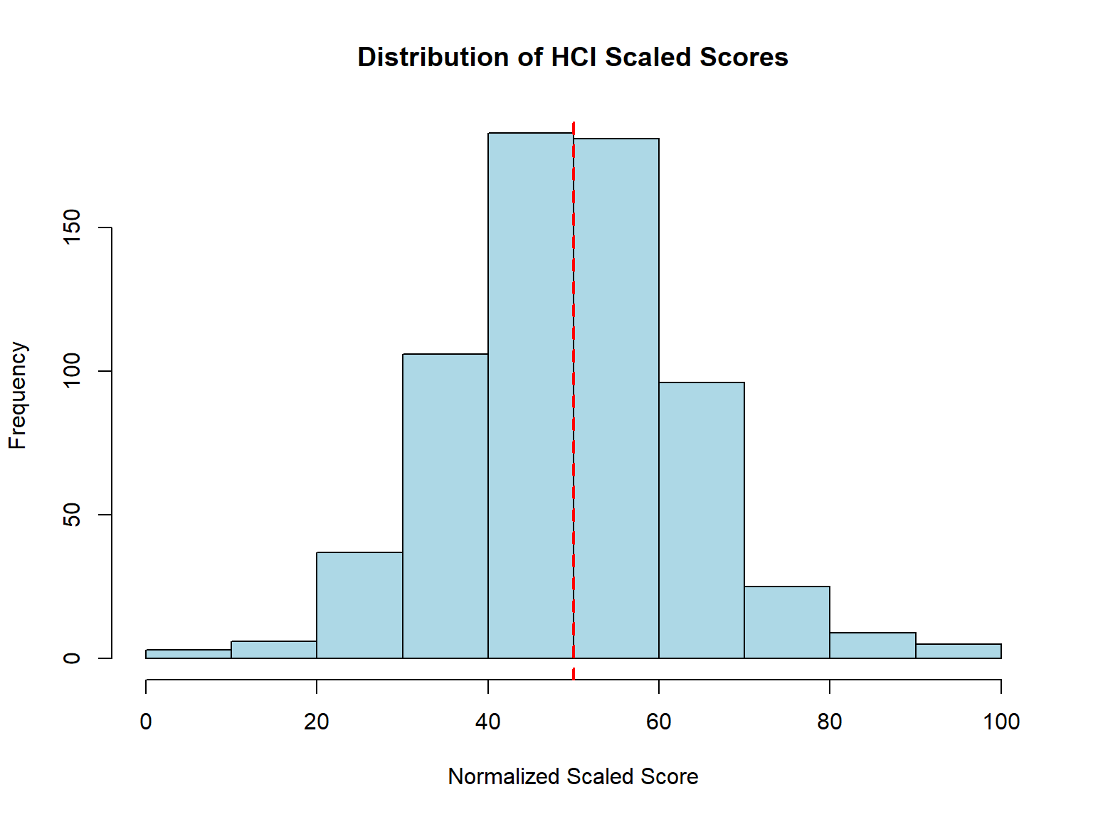
Item analysis
Now that we have the scored item responses, we will go ahead and
conduct item analysis for the hci dataset. First, we will check out the
correlations among the items using tetrachoric() function
from the psych package (note that we must use
tetrachoric correlations given that our items are dichotomously scored)
and then visualize the correlations using ggcorrplot().
ggcorrplot::ggcorrplot(corr = cormat_hci,
                       type = "lower",
                       show.diag = TRUE,
                       lab = TRUE,
lab_size = 3) 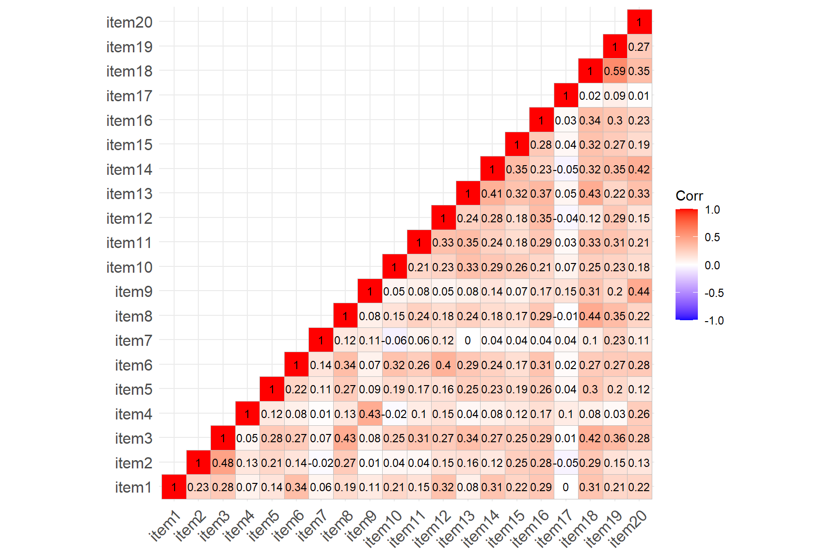
The correlation matrix plot shows that there are several problematic
items in the dataset, such as items 7 and 17. Next, we will use the
itemAnalysis() function from the CTT
package to run a more detailed item analysis for the scored hci
dataset.
# Run the item analysis and save it as hci_itemanalysis
hci_itemanalysis <- CTT::itemAnalysis(items = hci_items_scored, pBisFlag = .2, bisFlag = .2)

# Print the reliability
hci_itemanalysis
 Number of Items
 20

 Number of Examinees
 651

 Coefficient Alpha
0.715 itemName itemMean pBis bis alphaIfDeleted lowPBis lowBis
1 item1 0.6989247 0.28841909 0.37990903 0.7041972
2 item2 0.7526882 0.22061343 0.30125951 0.7099362
3 item3 0.8479263 0.35004183 0.53420292 0.7006955
4 item4 0.4039939 0.17298662 0.21914922 0.7150766 X
5 item5 0.4423963 0.27678377 0.34822354 0.7053505
6 item6 0.3625192 0.34188468 0.43826145 0.6991489
7 item7 0.5468510 0.10093796 0.12682596 0.7219621 X X
8 item8 0.7050691 0.32521530 0.42986414 0.7009218
9 item9 0.4331797 0.21296787 0.26829359 0.7114344
10 item10 0.6482335 0.26435677 0.34018971 0.7064185
11 item11 0.7788018 0.28511163 0.39841785 0.7046640
12 item12 0.5729647 0.31559335 0.39797842 0.7015908
13 item13 0.6082949 0.36121767 0.45898953 0.6972122
14 item14 0.7588326 0.33855783 0.46465921 0.7001197
15 item15 0.4439324 0.30056400 0.37806512 0.7030488
16 item16 0.6067588 0.38222680 0.48549208 0.6951640
17 item17 0.2964670 0.04340407 0.05732028 0.7253267 X X
18 item18 0.7972350 0.41712069 0.59412579 0.6943156
19 item19 0.7849462 0.36650603 0.51528308 0.6981434
20 item20 0.7219662 0.33955329 0.45348132 0.6997382 The results of our item analysis show that the internal consistency of the hci items is around 0.72 (not good enough for a summative assessment) and that three items (items 4, 7, and 17) have been flagged for showing low discrimination. We can see that item 17 is a very difficult item (\(p = 0.29\)) and both items7 and 17 have low discrimination. We can remove these two items from the test and rerun the item analysis:
# Run the item analysis and save it as hci_itemanalysis2
hci_itemanalysis2 <- CTT::itemAnalysis(items = hci_items_scored[, -c(7, 17)],
                                       pBisFlag = .2,
                                       bisFlag = .2)

# Print the reliability
hci_itemanalysis2
 Number of Items
 18

 Number of Examinees
 651

 Coefficient Alpha
0.733 itemName itemMean pBis bis alphaIfDeleted lowPBis lowBis
1 item1 0.6989247 0.2948723 0.3884093 0.7228366
2 item2 0.7526882 0.2352250 0.3212124 0.7278005
3 item3 0.8479263 0.3584801 0.5470807 0.7187943
4 item4 0.4039939 0.1703088 0.2157568 0.7347497 X
5 item5 0.4423963 0.2737195 0.3443684 0.7251008
6 item6 0.3625192 0.3401596 0.4360500 0.7186537
7 item8 0.7050691 0.3283374 0.4339909 0.7198352
8 item9 0.4331797 0.1987390 0.2503683 0.7322322 X
9 item10 0.6482335 0.2751882 0.3541283 0.7247489
10 item11 0.7788018 0.2894657 0.4045023 0.7232886
11 item12 0.5729647 0.3206200 0.4043173 0.7205367
12 item13 0.6082949 0.3715534 0.4721228 0.7155900
13 item14 0.7588326 0.3533586 0.4849728 0.7179002
14 item15 0.4439324 0.3061087 0.3850396 0.7219610
15 item16 0.6067588 0.3916629 0.4974776 0.7136207
16 item18 0.7972350 0.4246352 0.6048291 0.7125853
17 item19 0.7849462 0.3547787 0.4987953 0.7180327
18 item20 0.7219662 0.3423104 0.4571635 0.7186383 The updated item analysis results show that the internal consistency of the hci test increased to 0.73 (still not good but slightly better than the previous value). Although items 4 and 9 have been flagged for showing low point-biserial correlations, their pBis values are not too low. So, we can retain the remaining items on the test but remember that the overall internal consistency of this test is not sufficient for making summative evaluations or high-stakes decisions.
Standard error of measurement
An important test-level statistic for educational assessments is the standard error of measurement (SEM), which can be calculated as follows:
\[SEM = \sigma \sqrt{(1-r_{xx})},\] where \(\sigma\) is the standard deviation of the test scores and \(r_{xx}\) is the reliability of the test. In practice, SEM is often used to create a confidence interval around observed test scores scores. Calculating such confidence intervals allows us to capture the variability around the observe score and thereby explain where the true score corresponding to the observe score would be roughly located (with a certain level of confidence).
To calculate SEM and confidence intervals, we will create a custom
function that takes the item response data as an input and returns SEM
as well as confidence intervals for the total score. in the function, we
can specify the level of confidence we want (e.g.,
ci.level = 0.95 for 95% confidence intervals). The function
reports SEM, coefficient alpha, and the formula to calculate confidence
intervals. Also, it returns observed (raw) scores and their lower and
upper confidence intervals as a data frame.
# x is the response data
# ci.level is the confidence level we want
sem.ctt <- function(x, ci.level = 0.95) {
  require("CTT")
  rxx <- CTT::itemAnalysis(items = x)$alpha
  scores <- rowSums(x, na.rm = TRUE)
  sigma <- sd(scores, na.rm = TRUE)
  sem <- sigma*sqrt((1-rxx))
  z <- qnorm(1-(1-ci.level)/2)

  cat("****************************************************","\n")
  cat("","\n")
  cat(sprintf("%40s","Standard Error of Measurement"),"\n")
  cat("","\n")
  cat("****************************************************","\n")
  cat("","\n")
  cat("Coefficient alpha = ", rxx, "\n")
  cat("","\n")
  cat("Standard deviation = ", sigma, "\n")
  cat("","\n")
  cat("SEM = ", sem, "\n")
  cat("","\n")
  cat("To calculate confidence intervals with SEM, use:", "\n")
  cat("","\n")
  cat("Observed Score ± (", sem, "*", z, ")", "\n")
  cat("","\n")

  output <- data.frame(lower_CI = scores - (sem*z),
                       observed = scores,
                       upper_CI = scores + (sem*z))

  return(output)
}

# Calculate SEM
sem_hci <- sem.ctt(x = hci_items_scored, ci.level = 0.95)
****************************************************
Standard Error of Measurement
****************************************************
Coefficient alpha = 0.7154535
Standard deviation = 3.639684
SEM = 1.941513
To calculate confidence intervals with SEM, use:
Observed Score ± ( 1.941513 * 1.959964 )
  lower_CI observed upper_CI
1  12.1947       16  19.8053
2  15.1947       19  22.8053
3  13.1947       17  20.8053
4  16.1947       20  23.8053
5  15.1947       19  22.8053
6  16.1947       20  23.8053
Differential item functioning
Differential item functioning (DIF) is used in educational and psychological assessments to detect item-level bias. DIF occurs due to a conditional dependency between group membership of examinees (e.g., female vs. male) and item performance after controlling for the latent trait. As a result of DIF, a biased item provides either a constant advantage for a particular group (uniform DIF) or an advantage varying in magnitude and/or in direction across the latent trait continuum (nonuniform DIF). In the context of DIF, the focal group refers to the examinees who are suspected to be at a disadvantage compared to the examinees from the reference group when responding to the items on the test. If an item exhibits “uniform DIF”, then the performance of the focal group tends to be constantly worse than the performance of the reference group along the latent trait continuum. If the item exhibits “nonuniform DIF”, the difference between the focal and reference groups would not necessarily have a single direction.
The difR package (Magis et al., 2010) provides access to several methods for detecting dichotomous items exhibiting DIF. In the following example, we will use the Mantel-Haenszel (MH) and logistic regression methods to analyze the scored hci items in terms of DIF. We will use “gender” and “eng_first_lang” as group variables to identify the hci items that exhibit DIF based on gender or speaking English as a first language. To facilitate DIF analyses we will run in this part, I saved the scored items, gender, and eng_first_lang as hci_scored.csv. In addition, the R codes for the DIF analyses presented here are available here.
Now, let’s go head and import the data into R.
# Import the dataset
hci_scored <- read.csv("hci_scored.csv", header = TRUE)

# Print the first 6 rows of the dataset
head(hci_scored)
item1 item2 item3 item4 item5 item6 item7 item8 item9 item10 item11 item12 item13 item14 item15 item16
1 1 1 1 1 1 0 0 1 1 1 1 1 1 1 0 1
2 1 1 1 1 1 1 0 1 1 1 1 1 1 1 1 1
3 1 1 1 1 0 1 0 1 1 1 1 1 1 1 0 1
4 1 1 1 1 1 1 1 1 1 1 1 1 1 1 1 1
5 1 1 1 1 1 1 1 1 1 1 1 1 1 1 0 1
6 1 1 1 1 1 1 1 1 1 1 1 1 1 1 1 1
item17 item18 item19 item20 gender eng_first_lang
1 0 1 1 1 F yes
2 1 1 1 1 F yes
3 1 1 1 1 M yes
4 1 1 1 1 M yes
5 1 1 1 1 M yes
6 1 1 1 1 F yesNext, we will check the number of female/male students and students whose first language is English (or not).
  F   M
405 246
 no yes
143 508
In the following part, we will run DIF analysis to detect items with DIF based on gender and language. We will use female students as the focal group in gender-based DIF analysis and use students whose first language is not English as the focal group in language-based DIF analysis. Please note that males/those who speak English as their first language as the focal group would not change the results.
We will begin with the Mantel-Haenszel (MH) DIF method. The
difMH() function from the difR package
allows us to run the MF DIF method and detect items exhibiting DIF. The
function automatically calculates the total scores based on the response
data and use these scores to match the students based on their ability
levels when performing the MH test. However, we can also calculate the
total scores prior to DIF analysis and use it as the matching
variable.
Before we begin the analysis, let’s save the items in hci_scored, gender, and eng_first_lang as separate datasets.
# We will save the items, gender, and language as separate datasets
hci_items <- dplyr::select(hci_scored, starts_with("item"))

gender <- hci_scored$gender

language <- hci_scored$eng_first_lang
Now, let’s go ahead and run DIF analysis using the MH method for
gender and language. In the following example, we specify the items to
be tested for DIF (Data = hci_items), the group variable
(group = gender), the group (female) to be used as the
focal group (focal.name = "F"), and the matching variable
(match = "score") which automatically calculates the total
scores based on item responses (if we already have the total scores in
the data, then we can specify a variable name in the data for total test
scores). Also, we set purify = TRUE to run iterative
purification when conducting DIF analysis. With purification, items with
DIF are excluded from the calculation of the matching variable (i.e.,
total scores) and the analysis is rerun with clean items until no
further DIF items are detected.
# 1) Run the DIF analysis based on gender
gender_MH <- difR::difMH(Data = hci_items, # response data
                         group = gender, # group variable
                         focal.name = "F", # F for female students
                         match = "score", # matching variable
                         purify = TRUE) # if TRUE, purification is used

# Print the results
print(gender_MH)
Detection of Differential Item Functioning using Mantel-Haenszel method
with continuity correction and with item purification

Results based on asymptotic inference

Convergence reached after 2 iterations

Matching variable: test score

No set of anchor items was provided

No p-value adjustment for multiple comparisons

Mantel-Haenszel Chi-square statistic:

       Stat.  P-value
item1  5.1837 0.0228  *
item2  0.1790 0.6722
item3  0.0524 0.8189
item4  3.0679 0.0799  .
item5  0.4067 0.5237
item6  1.3774 0.2405
item7  0.2183 0.6403
item8  0.2457 0.6201
item9  1.6002 0.2059
item10 0.3804 0.5374
item11 0.0826 0.7738
item12 3.4527 0.0631  .
item13 0.0000 0.9948
item14 0.0000 0.9986
item15 0.2856 0.5931
item16 0.6194 0.4313
item17 0.0035 0.9529
item18 0.0081 0.9283
item19 5.1109 0.0238  *
item20 0.0161 0.8990

Signif. codes: 0 '***' 0.001 '**' 0.01 '*' 0.05 '.' 0.1 ' ' 1

Detection threshold: 3.8415 (significance level: 0.05)

Items detected as DIF items:

 item1
 item19


Effect size (ETS Delta scale):

Effect size code:
 'A': negligible effect
 'B': moderate effect
 'C': large effect

       alphaMH deltaMH
item1   0.6308  1.0827 B
item2   1.1173 -0.2606 A
item3   0.9044  0.2361 A
item4   0.7122  0.7975 A
item5   1.1387 -0.3053 A
item6   1.2749 -0.5708 A
item7   1.1015 -0.2272 A
item8   1.1325 -0.2924 A
item9   1.2767 -0.5741 A
item10  1.1484 -0.3252 A
item11  0.9152  0.2082 A
item12  0.6904  0.8706 A
item13  1.0213 -0.0496 A
item14  0.9757  0.0578 A
item15  0.8905  0.2725 A
item16  0.8404  0.4087 A
item17  1.0064 -0.0149 A
item18  0.9906  0.0223 A
item19  0.5729  1.3091 B
item20  1.0515 -0.1181 A

Effect size codes: 0 'A' 1.0 'B' 1.5 'C'
 (for absolute values of 'deltaMH')

Output was not captured! 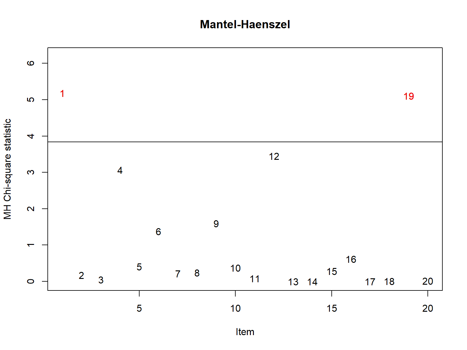
The plot was not captured!The output consists of two sections. The first part shows the MH chi-square statistics for the items and their corresponding p values. We see that two items (items 1 and 19) have been flagged at \(\alpha = .05\) for showing DIF between male and female students because their p values are less than .05. These items are also listed under “Items detected as DIF items”. The second part of the output shows the effect size using ETS delta classification. Two items (items 1 and 19) have been categorized as “B: Moderate DIF”, while the remaining items have been classified as “A: Negligible DIF”. There is no item with a “C: Large DIF” flag. The plot also shows the two items that have been flagged based on the MH chi-square test. These items appear above the horizontal line for the threshold chi-square value (\(\chi^2 = 3.84\) for the significance level of \(\alpha = .05\)).
Let’s also run the same type of analysis for language. This time we
only change the group variable as group = language.
# 2) Run the DIF analysis based on language
lang_MH <- difR::difMH(Data = hci_items, # response data
                       group = language, # group variable
                       focal.name = "no", # no for students whose first language is not English
                       match = "score", # matching variable
                       purify = TRUE) # if TRUE, purification is used

# Print the results
print(lang_MH)
Detection of Differential Item Functioning using Mantel-Haenszel method
with continuity correction and with item purification

Results based on asymptotic inference

Convergence reached after 2 iterations

Matching variable: test score

No set of anchor items was provided

No p-value adjustment for multiple comparisons

Mantel-Haenszel Chi-square statistic:

       Stat.  P-value
item1  1.5933 0.2069
item2  1.6164 0.2036
item3  4.3557 0.0369  *
item4  0.0003 0.9870
item5  0.3458 0.5565
item6  2.8791 0.0897  .
item7  0.0841 0.7718
item8  0.0191 0.8900
item9  0.0410 0.8396
item10 2.0092 0.1563
item11 0.0039 0.9499
item12 0.0091 0.9241
item13 0.2976 0.5854
item14 0.4777 0.4895
item15 0.0000 0.9980
item16 7.9690 0.0048  **
item17 0.2822 0.5953
item18 8.4877 0.0036  **
item19 1.1926 0.2748
item20 3.2762 0.0703  .

Signif. codes: 0 '***' 0.001 '**' 0.01 '*' 0.05 '.' 0.1 ' ' 1

Detection threshold: 3.8415 (significance level: 0.05)

Items detected as DIF items:

 item3
 item16
 item18


Effect size (ETS Delta scale):

Effect size code:
 'A': negligible effect
 'B': moderate effect
 'C': large effect

       alphaMH deltaMH
item1   0.7214  0.7676 A
item2   1.3642 -0.7298 A
item3   1.8628 -1.4619 B
item4   1.0290 -0.0671 A
item5   1.1615 -0.3518 A
item6   0.6357  1.0647 B
item7   1.0840 -0.1895 A
item8   0.9476  0.1264 A
item9   1.0698 -0.1585 A
item10  0.7198  0.7728 A
item11  1.0441 -0.1014 A
item12  1.0030 -0.0070 A
item13  1.1516 -0.3317 A
item14  1.2147 -0.4570 A
item15  1.0260 -0.0603 A
item16  0.5058  1.6018 C
item17  0.8636  0.3447 A
item18  0.4185  2.0468 C
item19  0.7499  0.6764 A
item20  1.5553 -1.0380 B

Effect size codes: 0 'A' 1.0 'B' 1.5 'C'
 (for absolute values of 'deltaMH')

Output was not captured! 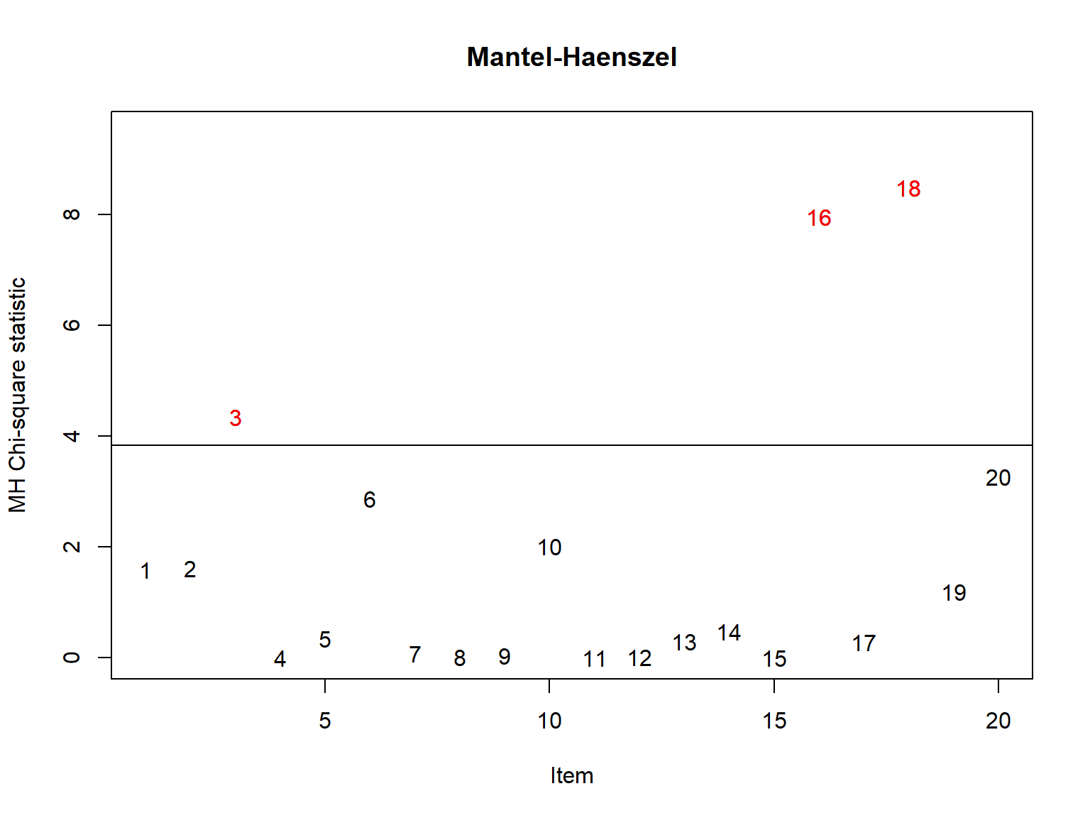
The plot was not captured!The results show that three items (item 3, 16, and 18) have been flagged for having language-based DIF. The effect size using ETS delta classification shows that item 3 has been classified as “B: Moderate DIF” whereas items 16 and 18 have been classified as “C: Large DIF”. In addition to these items, items 6 and 20 have been classified as “B: Moderate DIF”. Therefore, it would be worth examining the content of these items along with the other flagged items and determine why language-based DIF occurs.
The MH method is quite straightforward; however, it is not a powerful DIF method when it comes to detecting non-uniform DIF. In fact, the MH method cannot even distinguish what type of DIF (uniform or non-uniform) occurs in the items. To deal with these limitations, we will also repeat the same DIF analyses using the logistic regression (LR) method. This will allow us to validate our findings from the MH method and detect any additional items that we might have missed.
To implement the LR method, we will use the
difLogistic() function from the difR
package. The arguments for this function are nearly the same as those
for difMH(), except for type = "both" (which
is the default option) to run the DIF analysis for uniform and
nonuniform DIF. Alternatively, we could use either
type = "udif" or type = "nudif" to test the
items for only uniform or nonuniform DIF.
# 1) Run the DIF analysis based on gender
gender_LR <- difR::difLogistic(Data = hci_items, # response data
                               group = gender, # group variable
                               focal.name = "F", # F for female students
                               match = "score", # matching variable
                               type = "both", # Check both uniform and nonuniform DIF
                               purify = TRUE) # if TRUE, purification is used

# Print the results
print(gender_LR)
Detection of both types of Differential Item Functioning
using Logistic regression method, with item purification
and with LRT DIF statistic

Convergence reached after 1 iteration

Matching variable: test score

No set of anchor items was provided

No p-value adjustment for multiple comparisons

Logistic regression DIF statistic:

       Stat.   P-value
item1   7.9458  0.0188 *
item2   0.0069  0.9966
item3   0.7535  0.6861
item4   5.5434  0.0626 .
item5   0.2458  0.8844
item6   1.8683  0.3929
item7   0.2159  0.8977
item8   1.2364  0.5389
item9   4.0294  0.1334
item10  2.2201  0.3295
item11  4.7836  0.0915 .
item12  6.7575  0.0341 *
item13  1.9140  0.3840
item14  0.0040  0.9980
item15  0.8848  0.6425
item16  1.2484  0.5357
item17  0.3616  0.8346
item18  0.6338  0.7284
item19 11.3500  0.0034 **
item20  6.2415  0.0441 *

Signif. codes: 0 '***' 0.001 '**' 0.01 '*' 0.05 '.' 0.1 ' ' 1

Detection threshold: 5.9915 (significance level: 0.05)

Items detected as DIF items:

 item1
 item12
 item19
 item20


Effect size (Nagelkerke's R^2):

Effect size code:
 'A': negligible effect
 'B': moderate effect
 'C': large effect

       R^2    ZT JG
item1  0.0144 A  A
item2  0.0000 A  A
item3  0.0016 A  A
item4  0.0102 A  A
item5  0.0004 A  A
item6  0.0031 A  A
item7  0.0004 A  A
item8  0.0022 A  A
item9  0.0073 A  A
item10 0.0040 A  A
item11 0.0095 A  A
item12 0.0112 A  A
item13 0.0030 A  A
item14 0.0000 A  A
item15 0.0015 A  A
item16 0.0020 A  A
item17 0.0008 A  A
item18 0.0011 A  A
item19 0.0209 A  A
item20 0.0109 A  A

Effect size codes:
 Zumbo & Thomas (ZT): 0 'A' 0.13 'B' 0.26 'C' 1
 Jodoin & Gierl (JG): 0 'A' 0.035 'B' 0.07 'C' 1

Output was not captured! 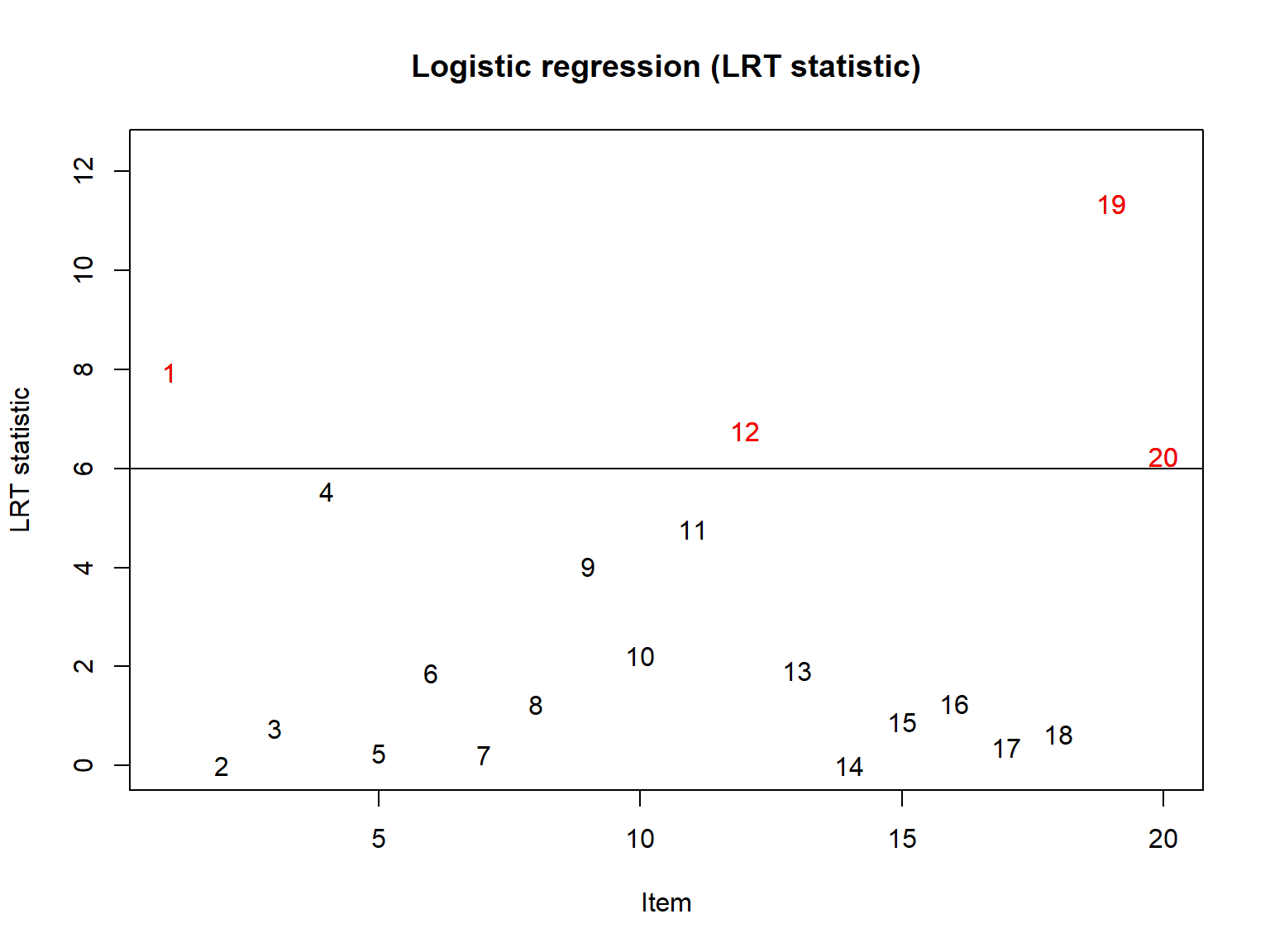
The plot was not captured!Similar to the output from the difMH() function, the
output from the difLogistic() function also consists of two
parts. The top part of the output shows the likelihood ratio test
statistics and corresponding p values for the items. In addition to
items 1 and 19), the LR method detected two more items with DIF, items
12 and 20, at the significance level of \(\alpha = .05\). The second part of the
output shows the effect sizes computed using the pseudo R-squared
differences. The results show that the effect size was “A: Negligible
DIF” for all of the items based on both effect size measures (ZT and
JG). In the plot, we see the four DIF items (items 1, 12, 19, and 20)
above the horizontal line for the threshold likelihood ratio statistic
(5.9915 for the significance level of \(\alpha
= .05\)).
The same plot() function can also be used for creating
individual plots for the flagged items based on the likelihood ratio
statistic. The plot creates separate item characteristic curves where
the x-axis is the total test scores and the y-axis shows the probability
of correct answer (i.e., receiving 1 over 0). This plot can indicate
whether the type of DIF is either uniform or nonuniform and which one of
the two groups (i.e., reference and focal) has the advantage over the
other group. In the following example, we will create item
characteristic curves for items 1 and 19. We specify the item using the
item argument and the plot type using
plot = "itemCurve".
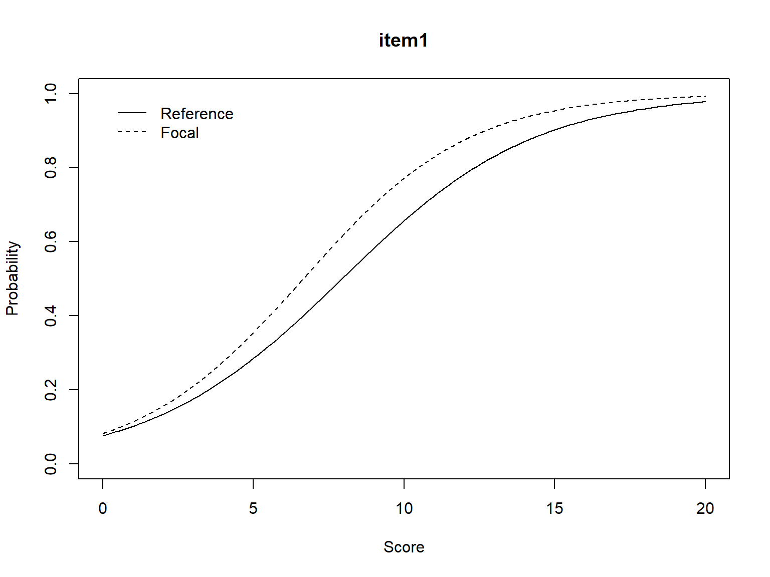
The plot was not captured!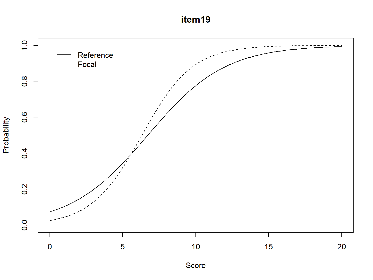
The plot was not captured!From the plots above, we can see that item 1 exhibits uniform DIF where the focal group (i.e., female students) are more likely to answer the item correctly compared to the reference group (i.e., male students). In other words, the item favors the female students. Unlike item 1, item 19 exhibits nonuniform DIF where the reference group is more likely to answer the item correctly until the total score of 5 but then the focal group becomes more advantageous among students with the total score > 5.
Now, we can repeat this process for language by replacing
group = gender with group = language.
# 2) Run the DIF analysis based on language
lang_LR <- difR::difLogistic(Data = hci_items, # response data
                             group = language, # group variable
                             focal.name = "no", # no for students whose first language is not English
                             match = "score", # matching variable
                             type = "both", # check both uniform and nonuniform DIF
                             purify = TRUE) # if TRUE, purification is used

# Print the results
print(lang_LR)
Detection of both types of Differential Item Functioning
using Logistic regression method, with item purification
and with LRT DIF statistic

Convergence reached after 4 iterations

Matching variable: test score

No set of anchor items was provided

No p-value adjustment for multiple comparisons

Logistic regression DIF statistic:

       Stat.   P-value
item1   6.8336  0.0328 *
item2   1.3503  0.5091
item3   3.0770  0.2147
item4   0.9306  0.6279
item5   2.2886  0.3184
item6   4.7808  0.0916 .
item7   3.5067  0.1732
item8   0.7884  0.6742
item9   5.3922  0.0675 .
item10  7.5287  0.0232 *
item11  0.0262  0.9870
item12  0.8611  0.6501
item13  7.1926  0.0274 *
item14  0.6589  0.7193
item15  0.0142  0.9929
item16 14.0757  0.0009 ***
item17  2.3535  0.3083
item18 13.1093  0.0014 **
item19  8.1858  0.0167 *
item20  2.1369  0.3435

Signif. codes: 0 '***' 0.001 '**' 0.01 '*' 0.05 '.' 0.1 ' ' 1

Detection threshold: 5.9915 (significance level: 0.05)

Items detected as DIF items:

 item1
 item10
 item13
 item16
 item18
 item19


Effect size (Nagelkerke's R^2):

Effect size code:
 'A': negligible effect
 'B': moderate effect
 'C': large effect

       R^2    ZT JG
item1  0.0121 A  A
item2  0.0027 A  A
item3  0.0067 A  A
item4  0.0016 A  A
item5  0.0039 A  A
item6  0.0079 A  A
item7  0.0065 A  A
item8  0.0014 A  A
item9  0.0094 A  A
item10 0.0134 A  A
item11 0.0001 A  A
item12 0.0014 A  A
item13 0.0115 A  A
item14 0.0012 A  A
item15 0.0000 A  A
item16 0.0219 A  A
item17 0.0049 A  A
item18 0.0243 A  A
item19 0.0152 A  A
item20 0.0037 A  A

Effect size codes:
 Zumbo & Thomas (ZT): 0 'A' 0.13 'B' 0.26 'C' 1
 Jodoin & Gierl (JG): 0 'A' 0.035 'B' 0.07 'C' 1

Output was not captured! 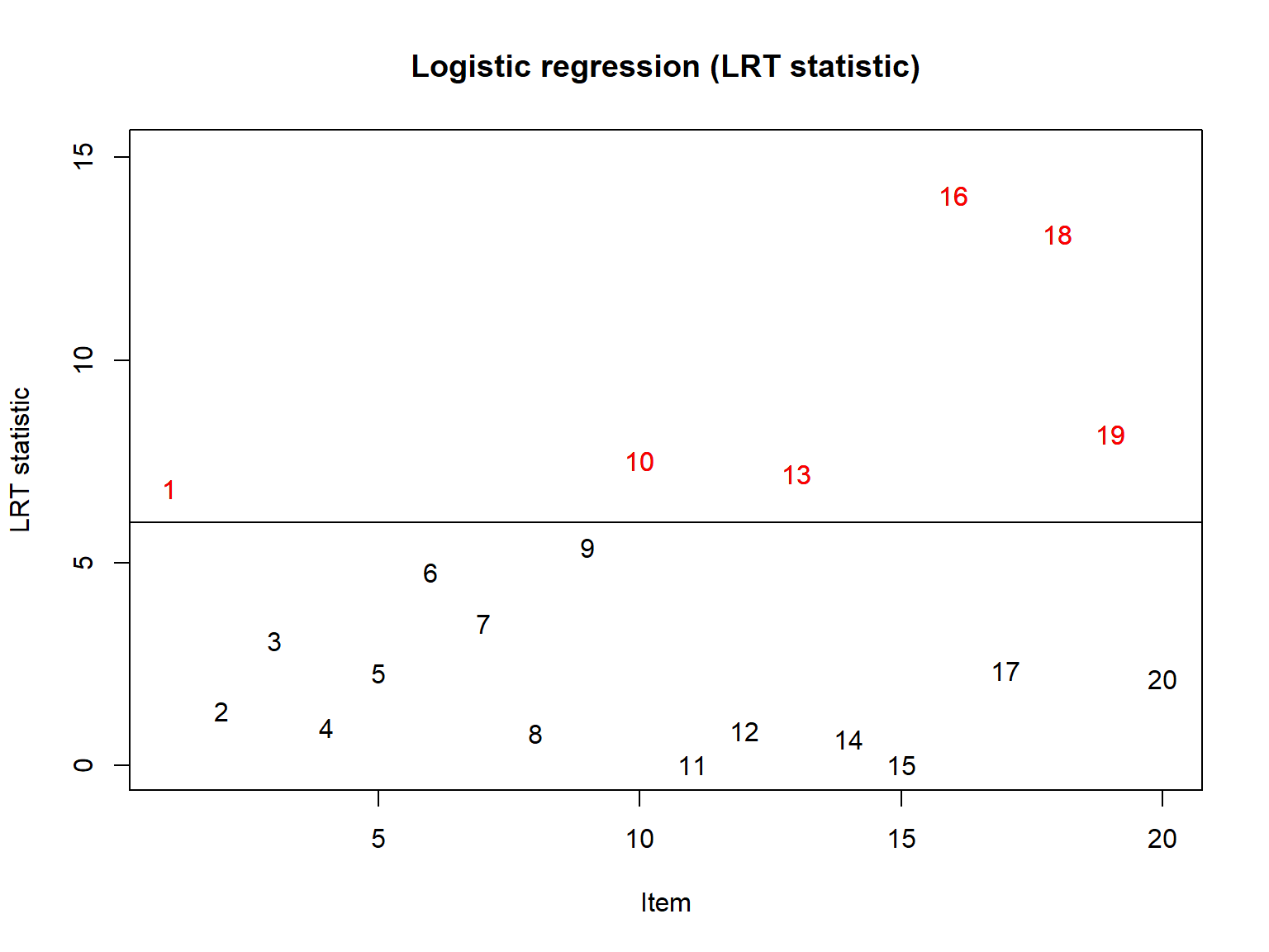
The plot was not captured!The LR method detected six items with language-based DIF: items 1, 10, 13, 16, 18, and 19. However, all of these items have the the effect size of “A: Negligible DIF” based on both effect size measures (ZT and JG). Finally, let’s take a look at two of the items that were flagged for having DIF. In the figures, we can see that item 16 a uniform DIF favoring the focal group whereas item 10 has a non-uniform DIF (i.e. which group is being favored depends on the total score on the test).
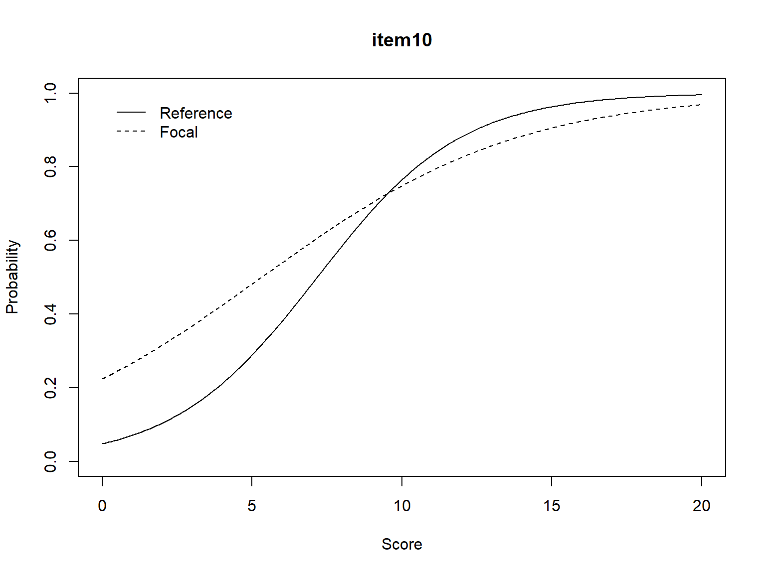
The plot was not captured!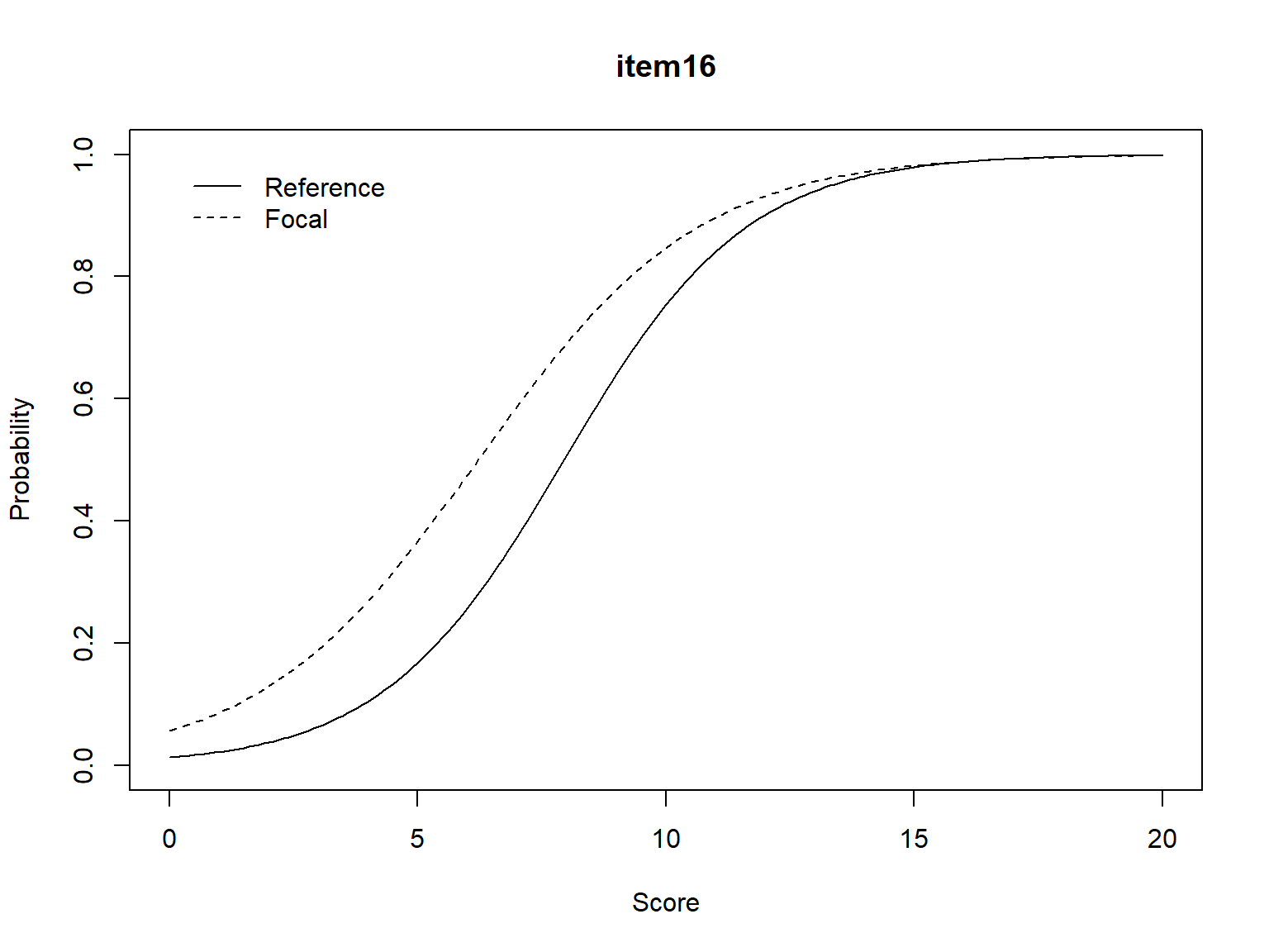
The plot was not captured!