2 Construct Validation

This chapter will focus on the evaluation of construct validity in educational and psychological instruments through factor analytic methods and psychometric network analysis.

2.1 Factor Analytic Methods

In this section, we will use factor exploratory factor analysis (EFA), confirmatory factor analysis (CFA), and principal component analysis (PCA) to evaluate the dimensionality of educational and psychological instruments. In the examples, we will use the following packages:

Table 2.1:
Package	URL
DataExplorer	http://CRAN.R-project.org/package=DataExplorer
ggcorrplot	http://CRAN.R-project.org/package=ggcorrplot
gridExtra	http://CRAN.R-project.org/package=gridExtra
psych	http://CRAN.R-project.org/package=psych
lavaan	http://CRAN.R-project.org/package=lavaan
semPlot	http://CRAN.R-project.org/package=semPlot
ggplot2	http://CRAN.R-project.org/package=ggplot2
mirt	http://CRAN.R-project.org/package=mirt
MASS	http://CRAN.R-project.org/package=MASS

We will install these packages using install.packages() and then activate them in our R session using library():

# Install the packages
install.packages(c("DataExplorer", "ggcorrplot", "gridExtra", "psych", "lavaan", "semPlot", 
                   "ggplot2", "mirt", "MASS"))

# Activate the required packages
library("DataExplorer") # for data summarization
library("ggcorrplot") # for creating correlation plots
library("gridExtra") # for placing multiple plots into a grid
library("psych") # for exploratory factor analysis
library("lavaan") # for confirmatory factor analysis
library("semPlot") # for creating path diagrams
library("ggplot2") # for general visualization tasks
library("mirt") # for simulating response data
library("MASS") # for simulating correlated multivariate data

Example 1: Synthetic Aperture Personality Assessment

In the first example, we will use the Synthetic Aperture Personality Assessment (SAPA)–a web-based personality assessment project (https://www.sapa-project.org/). The purpose of SAPA is to find patterns among the vast number of ways that people differ from one another in terms of their thoughts, feelings, interests, abilities, desires, values, and preferences (Condon & Revelle, 2014; Revelle et al., 2010). In this example, we will use a subset of SAPA (16 items) sampled from the full instrument (80 items) to develop online measures of ability. These 16 items measure four subskills (i.e., verbal reasoning, letter series, matrix reasoning, and spatial rotations) as part of the general intelligence, also known as g factor. The “sapa_data.csv” dataset is a data frame with 1525 individuals who responded to 16 multiple-choice items in SAPA. The original dataset is included in the psych package (Revelle, 2022). The dataset can be downloaded from sapa_data.csv. In addition, the R codes for the analyses presented in this section are available in example1.R.

Exploratory Data Analysis

We will begin our analysis by conducting exploratory data analysis (EDA). As you may remember from the CTT section, we use EDA to check the quality of our data and identify potential problems (i.e., missing values) in the data. In this section, we will import sapa_data.csv into R and review the variables in the dataset using descriptive statistics and visualizations.

First, we will import the data into R using the read.csv() function and save it as “sapa”.

sapa <- read.csv("sapa_data.csv", header = TRUE)

Using the head() function, we can now view the first 6 rows of the sapa dataset:

head(sapa)

  reason.4 reason.16 reason.17 reason.19 letter.7 letter.33 letter.34 letter.58 matrix.45 matrix.46 matrix.47
1        0         0         0         0        0         1         0         0         0         0         0
2        0         0         1         0        1         0         1         0         0         0         0
3        0         1         1         0        1         0         0         0         1         1         0
4        1         0         0         0        0         0         1         0         0         0         0
5        0         1         1         0        0         1         0         0         1         1         0
6        1         1         1         1        1         1         1         1         1         1         1
  matrix.55 rotate.3 rotate.4 rotate.6 rotate.8
1         1        0        0        0        0
2         0        0        0        1        0
3         0        0        0        0        0
4         0        0        0        0        0
5         0        0        0        0        0
6         0        1        1        1        0

The dataset consists of 1525 rows (i.e., examinees) and 16 variables (i.e., SAPA items). We can get more information on the dataset using the introduce() and plot_intro() functions from the DataExplorer package (Cui, 2020):

DataExplorer::introduce(sapa)

DataExplorer::plot_intro(sapa)


rows	1,525
columns	16
discrete_columns	0
continuous_columns	16
all_missing_columns	0
total_missing_values	25
complete_rows	1,523
total_observations	24,400
memory_usage	101,832

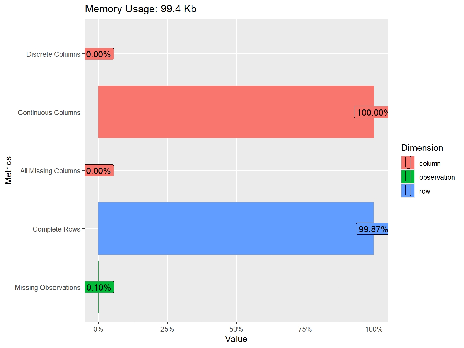
The plot above shows that all of the variables in the dataset are continuous. We also see that some of the variables have missing values but the proportion of missing data is very small (only 0.10%). To have a closer look at missing values, we can visualize the proportion of missingness for each variable using plot_missing() from DataExplorer.

DataExplorer::plot_missing(sapa)

As we analyze the sapa dataset, we may start with the assumption that all SAPA items measure the same latent trait (general intelligence or g). However, given that the items come from different content areas (i.e., verbal reasoning, letter series, matrix reasoning, and spatial rotations), we must ensure that these items are sufficiently correlated with each other.

Since the SAPA items are dichotomously scored (i.e., 0: incorrect and 1: correct), we cannot use Pearson correlations, which could be obtained using the cor() function in R. Instead, we will compute the inter-item correlations among the SAPA items using the tetrachoric() function from psych and then extract “rho” (i.e., the correlation matrix of the items).

# Save the correlation matrix
cormat <- psych::tetrachoric(x = sapa)$rho

# Print the correlation matrix
print(cormat)

	reason.4	reason.16	reason.17	reason.19	letter.7	letter.33	letter.34	letter.58	matrix.45	matrix.46	matrix.47	matrix.55	rotate.3	rotate.4	rotate.6	rotate.8
reason.4	1.000	0.474	0.600	0.484	0.462	0.380	0.479	0.455	0.431	0.399	0.401	0.299	0.456	0.491	0.447	0.436
reason.16	0.474	1.000	0.536	0.458	0.471	0.374	0.449	0.380	0.351	0.337	0.421	0.314	0.327	0.443	0.408	0.364
reason.17	0.600	0.536	1.000	0.550	0.473	0.440	0.473	0.480	0.358	0.392	0.466	0.316	0.386	0.427	0.506	0.401
reason.19	0.484	0.458	0.550	1.000	0.434	0.435	0.465	0.423	0.383	0.323	0.407	0.306	0.364	0.419	0.369	0.333
letter.7	0.462	0.471	0.473	0.434	1.000	0.538	0.603	0.523	0.342	0.412	0.442	0.279	0.328	0.443	0.364	0.275
letter.33	0.380	0.374	0.440	0.435	0.538	1.000	0.574	0.448	0.335	0.397	0.392	0.318	0.340	0.394	0.369	0.268
letter.34	0.479	0.449	0.473	0.465	0.603	0.574	1.000	0.515	0.365	0.436	0.481	0.256	0.374	0.416	0.348	0.308
letter.58	0.455	0.380	0.480	0.423	0.523	0.448	0.515	1.000	0.330	0.342	0.385	0.371	0.416	0.457	0.439	0.397
matrix.45	0.431	0.351	0.358	0.383	0.342	0.335	0.365	0.330	1.000	0.511	0.403	0.348	0.307	0.328	0.266	0.309
matrix.46	0.399	0.337	0.392	0.323	0.412	0.397	0.436	0.342	0.511	1.000	0.383	0.252	0.287	0.323	0.350	0.290
matrix.47	0.401	0.421	0.466	0.407	0.442	0.392	0.481	0.385	0.403	0.383	1.000	0.362	0.407	0.402	0.341	0.342
matrix.55	0.299	0.314	0.316	0.306	0.279	0.318	0.256	0.371	0.348	0.252	0.362	1.000	0.327	0.323	0.300	0.341
rotate.3	0.456	0.327	0.386	0.364	0.328	0.340	0.374	0.416	0.307	0.287	0.407	0.327	1.000	0.771	0.665	0.675
rotate.4	0.491	0.443	0.427	0.419	0.443	0.394	0.416	0.457	0.328	0.323	0.402	0.323	0.771	1.000	0.691	0.682
rotate.6	0.447	0.408	0.506	0.369	0.364	0.369	0.348	0.439	0.266	0.350	0.341	0.300	0.665	0.691	1.000	0.665
rotate.8	0.436	0.364	0.401	0.333	0.275	0.268	0.308	0.397	0.309	0.290	0.342	0.341	0.675	0.682	0.665	1.000

The correlation matrix above does not show any negative or low correlations–which is a very good sign 👍!!! To check the associations among the items more carefully, we will also create a correlation matrix plot using the ggcorrplot() function from the ggcorrplot package (Kassambara, 2023). We will include the hc.order = TRUE argument to perform hierarchical clustering. This will look for groups (i.e., clusters) of items that are strongly associated with each other. If all SAPA items measure the same latent trait, we should see a single cluster of items.

ggcorrplot::ggcorrplot(corr = cormat, # correlation matrix
                       type = "lower", # print only the lower part of the correlation matrix
                       hc.order = TRUE, # hierarchical clustering
                       show.diag = TRUE, # show the diagonal values of 1
                       lab = TRUE, # add correlation values as labels
                       lab_size = 3) # Size of the labels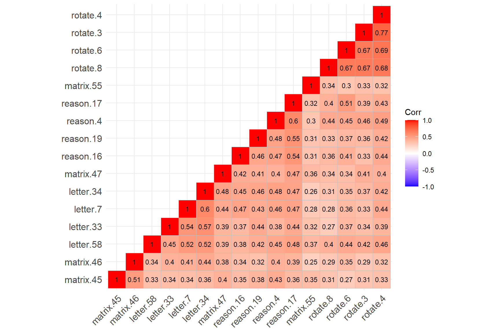

The figure above shows that the four rotation items have created a cluster (see the cluster on the top-right corner), while the remaining SAPA items have created another cluster (see the cluster on the bottom-left corner). The rotation items are strongly correlated with each other (not surprising given that they all focus on the rotation skills); however, the same items have relatively lower correlations with the other items in the dataset. Also, matrix.55 seems to have relatively low correlations with the items from both clusters.

The findings of hierarchical clustering suggest that the SAPA items may not necessarily be measuring a single latent trait. The items are very likely to be multidimensional. However, hierarchical clustering is not a direct test of dimensionality. To ensure that there is a single factor (i.e., latent trait) underlying the SAPA items, we need to perform factor analysis and evaluate the factor structure of the SAPA items (i.e., dimensionality).

Exploratory Factor Analysis

Factor analysis is a widely-used statistical technique that aims to explain the common variability among a set of observed variables and transform the variables into a reduced set of variables known as factors (or dimensions). At the core of factor analysis is the desire to reduce the dimensionality of the data from $p$ observed variables to $q$ factors, such that $q < p$. During instrument development or when there are no prior beliefs about the dimensionality of an existing instrument, exploratory factor analysis (EFA) should be considered to investigate the factorial structure of the instrument. To perform EFA, we need to specify the number of factors to extract, how to rotate factors (if the expected number of factors > 1), and which type of estimation method should be used depending on the nature of the data (i.e., categorical, ordinal, or continuous).

The psych package includes several functions to perform EFA with different estimation methods. In this example, we will use the fa() function in the psych package to perform EFA. To use the function, we need to specify the following items:

r = Response data (either raw data or a correlation matrix)
n.obs = Number of observations in the data (necessary only when using a correlation matrix)
nfactors = Number of factors that we expect to find in the data
rotate = Type of rotation if $n > 1$. We can use “varimax” for an orthogonal rotation that assumes no correlation between factors or “oblimin” for an oblique rotation that assumes factors are somewhat correlated
fm = Factor analysis method. We will use “ml” (i.e., maximum likelihood estimation) for EFA
cor = How to find the correlations when using raw data. For continuous variable, use cor = "Pearson" (Pearson correlation); for dichotomous variables, use cor = "tet" (tetrachoric correlation); for polytomous variables (e.g., Likert scales), use cor = "poly" (polychoric correlation).

First, we will try a one-factor model, evaluate model fit, and determine whether a one-factor (i.e., unidimensional) structure is acceptable for the SAPA items:

# Try one-factor EFA model --> nfactors = 1
efa.model1 <- psych::fa(r = sapa, nfactors = 1, fm = "ml", cor = "tet")

# Print the results 
print(efa.model1, sort = TRUE) # Show the factor loadings sorted by absolute value

Factor Analysis using method =  ml
Call: psych::fa(r = sapa, nfactors = 1, fm = "ml", cor = "tet")
Standardized loadings (pattern matrix) based upon correlation matrix
           V  ML1   h2   u2 com
rotate.4  14 0.75 0.57 0.43   1
reason.17  3 0.71 0.50 0.50   1
rotate.6  15 0.70 0.50 0.50   1
reason.4   1 0.70 0.49 0.51   1
rotate.3  13 0.70 0.48 0.52   1
letter.34  7 0.67 0.45 0.55   1
letter.58  8 0.66 0.43 0.57   1
letter.7   5 0.66 0.43 0.57   1
rotate.8  16 0.66 0.43 0.57   1
reason.19  4 0.63 0.40 0.60   1
reason.16  2 0.63 0.40 0.60   1
matrix.47 11 0.61 0.38 0.62   1
letter.33  6 0.61 0.38 0.62   1
matrix.46 10 0.54 0.30 0.70   1
matrix.45  9 0.53 0.28 0.72   1
matrix.55 12 0.47 0.22 0.78   1

                ML1
SS loadings    6.64
Proportion Var 0.42

Mean item complexity =  1
Test of the hypothesis that 1 factor is sufficient.

The degrees of freedom for the null model are  120  and the objective function was  8.04 with Chi Square of  12198
The degrees of freedom for the model are 104  and the objective function was  1.85 

The root mean square of the residuals (RMSR) is  0.08 
The df corrected root mean square of the residuals is  0.09 

The harmonic number of observations is  1523 with the empirical chi square  2331  with prob <  0 
The total number of observations was  1525  with Likelihood Chi Square =  2801  with prob <  0 

Tucker Lewis Index of factoring reliability =  0.742
RMSEA index =  0.13  and the 90 % confidence intervals are  0.126 0.135
BIC =  2039
Fit based upon off diagonal values = 0.96
Measures of factor score adequacy             
                                                   ML1
Correlation of (regression) scores with factors   0.96
Multiple R square of scores with factors          0.92
Minimum correlation of possible factor scores     0.85

The output shows the factor loadings for each item (see the ML1 column referring the first factor produced by the maximum likelihood (ML) method) and the proportion of explained variance (42%; see Proportion Var). The factor loadings seem to be high enough based on the rule of thumb of $\lambda \geq 0.3$. We can determine model fit based on model fit indices of root mean square of residuals (RMSR), root mean square error of approximation (RMSEA), and Tucker-Lewis Index. We can use Hu & Bentler (1999)’s guidelines for these model fit indices: Tucker-Lewis index (TLI) > .95, RMSEA < .06, and RMSR near zero indicate good model fit. The fit measures in the output show that the one-factor model does not necessarily fit the sapa dataset very well.

In the output, $h^2$ shows the amount of variance in the item/variable explained by the (retained) factors. It is the sum of the squared loadings (i.e., communality), $u^2$, which is $1 - h^2$, shows residual variance (i.e., uniqueness), and com (i.e., item complexity = ${(Σ λ_i^2)^2}/{Σ λ_i^4}$ where $\lambda_i$ is the factor loading on the $i^{th}$ factor) shows how much an item reflects a single construct (e.g., com equals 1 if an item loads only on one factor, 2 if evenly loads on two factors, etc.).

If we wanted to report the chi-square ($\chi^2$) test for our model, we would use the following part in the output: The total number of observations was 1525 with Likelihood Chi Square = 2801 with prob < 0. We can also extract these values from the model using efa.model1$STATISTIC, efa.model1$dof, efa.model1$PVAL,

Next, we will fit a two-factor model to the sapa dataset by using nfactors = 2:

# Try two-factor EFA model --> nfactors=2
efa.model2 <- psych::fa(sapa, nfactors = 2, rotate = "oblimin", fm = "ml", cor = "tet")

# Print the results 
print(efa.model2, sort = TRUE)

Factor Analysis using method =  ml
Call: psych::fa(r = sapa, nfactors = 2, rotate = "oblimin", fm = "ml", 
    cor = "tet")
Standardized loadings (pattern matrix) based upon correlation matrix
          item   ML1   ML2   h2   u2 com
letter.34    7  0.80 -0.09 0.56 0.44 1.0
letter.7     5  0.78 -0.08 0.54 0.46 1.0
letter.33    6  0.70 -0.05 0.45 0.55 1.0
reason.17    3  0.67  0.08 0.52 0.48 1.0
reason.19    4  0.63  0.04 0.43 0.57 1.0
reason.16    2  0.60  0.07 0.42 0.58 1.0
matrix.46   10  0.59 -0.01 0.34 0.66 1.0
matrix.47   11  0.58  0.08 0.40 0.60 1.0
letter.58    8  0.57  0.14 0.45 0.55 1.1
reason.4     1  0.57  0.18 0.49 0.51 1.2
matrix.45    9  0.54  0.02 0.30 0.70 1.0
matrix.55   12  0.34  0.17 0.22 0.78 1.5
rotate.3    13 -0.04  0.89 0.74 0.26 1.0
rotate.8    16 -0.04  0.83 0.64 0.36 1.0
rotate.4    14  0.08  0.82 0.77 0.23 1.0
rotate.6    15  0.08  0.74 0.64 0.36 1.0

                       ML1  ML2
SS loadings           4.88 3.01
Proportion Var        0.31 0.19
Cumulative Var        0.31 0.49
Proportion Explained  0.62 0.38
Cumulative Proportion 0.62 1.00

 With factor correlations of 
     ML1  ML2
ML1 1.00 0.64
ML2 0.64 1.00

Mean item complexity =  1.1
Test of the hypothesis that 2 factors are sufficient.

The degrees of freedom for the null model are  120  and the objective function was  8.04 with Chi Square of  12198
The degrees of freedom for the model are 89  and the objective function was  0.64 

The root mean square of the residuals (RMSR) is  0.04 
The df corrected root mean square of the residuals is  0.05 

The harmonic number of observations is  1523 with the empirical chi square  564  with prob <  4.3e-70 
The total number of observations was  1525  with Likelihood Chi Square =  969  with prob <  7.1e-148 

Tucker Lewis Index of factoring reliability =  0.902
RMSEA index =  0.081  and the 90 % confidence intervals are  0.076 0.085
BIC =  317
Fit based upon off diagonal values = 0.99
Measures of factor score adequacy             
                                                   ML1  ML2
Correlation of (regression) scores with factors   0.95 0.95
Multiple R square of scores with factors          0.90 0.91
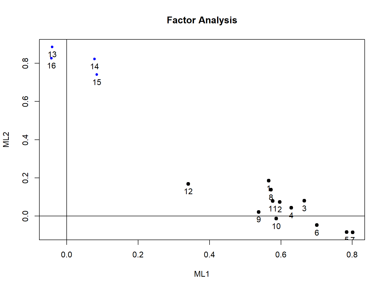
Minimum correlation of possible factor scores     0.81 0.82

Based on the factor loadings listed under the ML1 and ML2 columns, we see that the first 12 items are highly loaded on the first factor whereas the last four items (i.e., rotation items) are highly loaded on the second factor. This finding is aligned with what we have observed in the correlation matrix plot earlier.

We can also visualize the factor loadings using a bar plot. Below we will define a custom function that will take the results of EFA returned from the psych::fa function and create bar plots for each variable based on the values of factor loadings. To identify the important loadings more easily, we will use blue for factor loadings > 0.3 and lightgray for smaller loadings.

# Define the function
barplot_EFA <- function(model) {
  require("ggplot2")
  require("gridExtra")
  
  loadings <- model$loadings
  
  plots <- lapply(1:ncol(loadings), function(i) {
    ggplot2::ggplot(data.frame(Variables = rownames(loadings), Loading = loadings[, i], Highlight = abs(loadings[, i]) >= 0.3), 
           aes(x = Variables, y = Loading, fill = Highlight)) +
      ggplot2::geom_bar(stat = "identity", show.legend = FALSE) +
      ggplot2::scale_fill_manual(values = c("TRUE" = "blue", "FALSE" = "lightgray")) +
      ggplot2::ggtitle(paste("Factor", i)) +
      ggplot2::theme_bw() +
      ggplot2::theme(axis.text.x = element_text(angle = 45, hjust = 1)) +
      ggplot2::labs(caption = "Note: Blue bars represent loadings >= 0.3; Gray bars represent loadings < 0.3.") +
      ggplot2::scale_y_continuous(limits = c(-1, 1), breaks = seq(-1, 1, by = 0.25))
  })
  
  do.call(gridExtra::grid.arrange, c(plots, ncol = 2))
}


# Run the function for the two-factor model
barplot_EFA(efa.model2)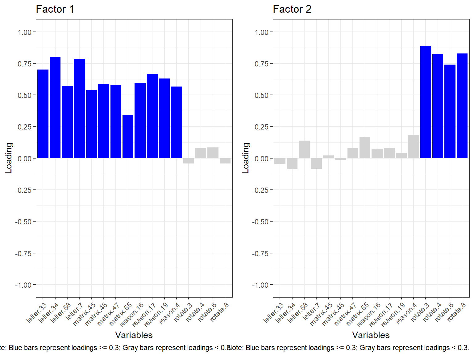

The bar plot above also shows that the first 12 items are loaded on Factor 1 while the remaining 4 items focused on rotation are loaded on Factor 2. To better understand if this structure is meaningful, we need to continue reviewing the statistical output we printed earlier for efa.model2.

The rest of the output shows that the first factor explains 31% of the total variance while the second factor explains 19% of the total variance (see Proportion Var). Compared to the one-factor model, the two-factor model explains an additional 8% of variance in the data. The two factors seem to be moderately correlated ($r = .64$). The model fit indices show that the two-factor model fits the data better, although the model fit indices still do not entirely meet the criteria for sufficient model fit. We can plot the factor loadings to get a sense of how the items relate to the two factors (note that this plot becomes much more complex as we plot 3 or more factors).

plot(efa.model2)

So far, the one-factor and two-factor models did not seem to fit the data adequately. The two-factor model separated the rotation items from the rest of the SAPA items. Do we expect to find four meaningful factors based on each domain covered in the SAPA items (i.e., verbal reasoning, letter series, matrix reasoning, and spatial rotations)? If this is the case, we can try a four-factor model and evaluate the fit and factor loadings for this model.

# Try four-factor EFA model --> nfactors=4
efa.model4 <- psych::fa(sapa, nfactors = 4, rotate = "oblimin", fm = "ml", cor = "tet")

# Print the results 
print(efa.model4, sort = TRUE)

Factor Analysis using method =  ml
Call: psych::fa(r = sapa, nfactors = 4, rotate = "oblimin", fm = "ml", 
    cor = "tet")
Standardized loadings (pattern matrix) based upon correlation matrix
          item   ML3   ML4   ML1   ML2   h2    u2 com
rotate.3    13  0.88  0.03 -0.08  0.02 0.75 0.254 1.0
rotate.4    14  0.84  0.14 -0.07 -0.01 0.78 0.216 1.1
rotate.8    16  0.80 -0.13  0.08  0.06 0.65 0.353 1.1
rotate.6    15  0.72 -0.03  0.21 -0.05 0.66 0.345 1.2
letter.34    7 -0.01  0.79  0.00  0.01 0.64 0.365 1.0
letter.7     5 -0.01  0.76  0.03 -0.01 0.60 0.399 1.0
letter.33    6  0.02  0.66  0.02  0.02 0.49 0.507 1.0
letter.58    8  0.18  0.46  0.12  0.01 0.45 0.547 1.5
matrix.47   11  0.12  0.34  0.15  0.16 0.39 0.608 2.1
reason.17    3  0.00  0.03  0.89  0.01 0.83 0.167 1.0
reason.4     1  0.19  0.17  0.38  0.15 0.51 0.486 2.3
reason.19    4  0.07  0.28  0.34  0.11 0.44 0.563 2.3
reason.16    2  0.10  0.27  0.34  0.07 0.42 0.579 2.2
matrix.45    9  0.00 -0.01 -0.01  0.97 0.92 0.078 1.0
matrix.46   10  0.02  0.29  0.08  0.35 0.38 0.616 2.1
matrix.55   12  0.19  0.13  0.09  0.20 0.23 0.775 3.1

                       ML3  ML4  ML1  ML2
SS loadings           3.12 2.83 1.77 1.43
Proportion Var        0.19 0.18 0.11 0.09
Cumulative Var        0.19 0.37 0.48 0.57
Proportion Explained  0.34 0.31 0.19 0.16
Cumulative Proportion 0.34 0.65 0.84 1.00

 With factor correlations of 
     ML3  ML4  ML1  ML2
ML3 1.00 0.53 0.53 0.38
ML4 0.53 1.00 0.63 0.48
ML1 0.53 0.63 1.00 0.41
ML2 0.38 0.48 0.41 1.00

Mean item complexity =  1.6
Test of the hypothesis that 4 factors are sufficient.

The degrees of freedom for the null model are  120  and the objective function was  8.04 with Chi Square of  12198
The degrees of freedom for the model are 62  and the objective function was  0.23 

The root mean square of the residuals (RMSR) is  0.02 
The df corrected root mean square of the residuals is  0.03 

The harmonic number of observations is  1523 with the empirical chi square  163  with prob <  4.5e-11 
The total number of observations was  1525  with Likelihood Chi Square =  355  with prob <  9.6e-43 

Tucker Lewis Index of factoring reliability =  0.953
RMSEA index =  0.056  and the 90 % confidence intervals are  0.05 0.061
BIC =  -99.1
Fit based upon off diagonal values = 1
Measures of factor score adequacy             
                                                   ML3  ML4  ML1  ML2
Correlation of (regression) scores with factors   0.96 0.93 0.93 0.96
Multiple R square of scores with factors          0.91 0.86 0.87 0.93
Minimum correlation of possible factor scores     0.83 0.72 0.74 0.85

The four-factor model yielded the best model fit results: $RMSEA = 0.056$, $RMSR = 0.02$, and Tucker Lewis Index is 0.953. However, our assumption of creating a separate factor for each domain did not entirely hold. The output shows that matrix.47 is mostly loaded on ML4 with the letter series items, and matrix.55 is not sufficiently loaded on any of the factors. At this point, we need to make a theoretical decision informed by the statistical output. Should we keep the matrix reasoning items in the dataset and use the four-factor model? Or, instead, can we remove the matrix items from the dataset and evaluate the factor structure with the remaining items (assuming three factors)? We could also fit a four-factor CFA model to the data to investigate the model fit based on the theoretical model that the items of each domain define a separate factor (i.e., forcing the matrix items to create a matrix reasoning factor, verbal reasoning items to create a verbal reasoning factor, and so on).

Now, let’s see the scree plot for the four-factor model. We will extract the eigenvalues from the common factor solution, create a separate dataset with them, and then visualize the values in a scree plot:

data_eigen <- data.frame(ev = efa.model4$values, 
                         # 16 eigenvalues due to having 16 items in SAPA
                         factor_number=factor(1:16)) 

ggplot2::ggplot(data_eigen, 
                aes(x = factor_number, y = ev, group = 1)) + 
  geom_point() + 
  geom_line() +
  theme_bw(base_size=15) +
  xlab("Factor number") + 
  ylab("Eigenvalue")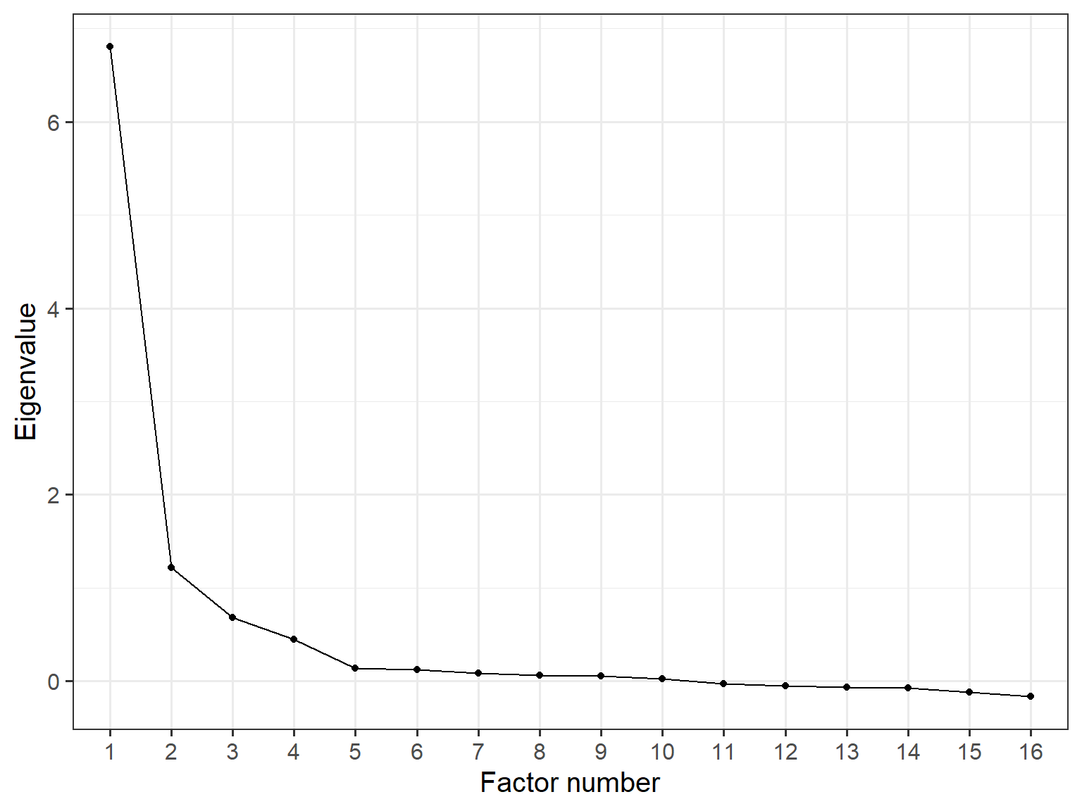

As the scree plot demonstrates, identifying a clear breaking (or elbow) point is quite difficult. In our example, if we accept the 4th point as the elbow point, then the scree plot suggests that the model should have four factors. However, there is a less pronounced slope change between 3 and 4 factors. So, the scree plot might lead us to consider either three- or four-factor solutions. At this point, the interpretability of the extracted factors and their factor loadings may serve as better criteria in the selection of a meaningful factor solution.

The psych package also includes an omega ($\omega$) function that fits a bi-factor EFA model to the data. This particular model assumes that there is a general factor associated with every item, as well as unique factors based on the constructs underlying the items. So, the function performs hierarchical factor analysis in the background, without requiring an explicit definition of the bi-factor structure.

Since the SAPA items are expected to measure the general intelligence (g), we can assume that each domain (verbal reasoning, letter series, matrix reasoning, and spatial rotations) will define a separate factor but all the SAPA items will define the general intelligence.

# Bi-factor EFA model
omega.model <- psych::omega(sapa, nfactors = 4, fm = "ml", poly = TRUE)

# Print the results 
print(omega.model)

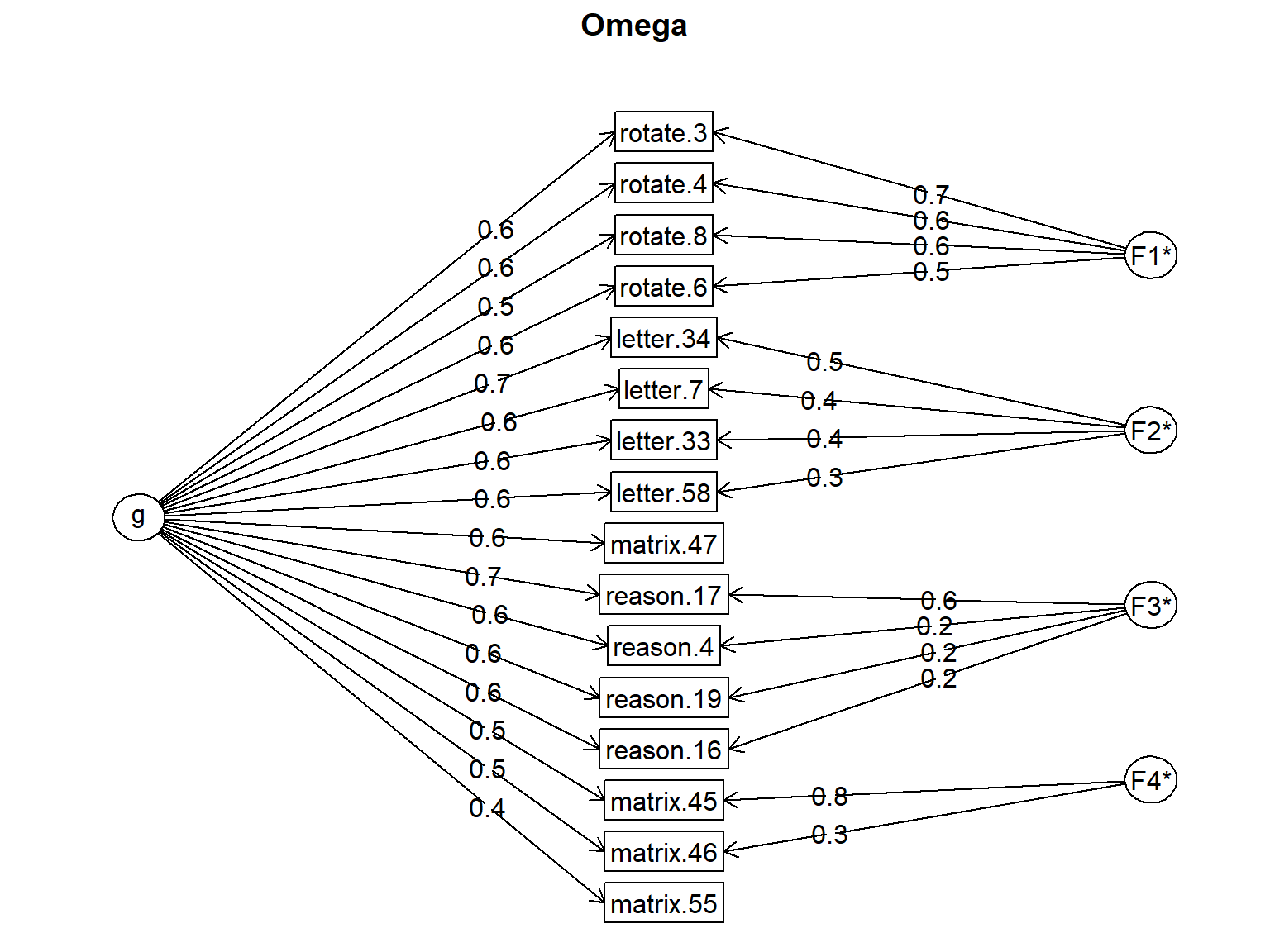
Omega 
Call: omegah(m = m, nfactors = nfactors, fm = fm, key = key, flip = flip, 
    digits = digits, title = title, sl = sl, labels = labels, 
    plot = plot, n.obs = n.obs, rotate = rotate, Phi = Phi, option = option, 
    covar = covar)
Alpha:                 0.92 
G.6:                   0.93 
Omega Hierarchical:    0.76 
Omega H asymptotic:    0.8 
Omega Total            0.94 

Schmid Leiman Factor loadings greater than  0.2 
             g   F1*   F2*   F3*   F4*   h2   u2   p2
reason.4  0.64              0.24       0.51 0.49 0.80
reason.16 0.59              0.21       0.42 0.58 0.81
reason.17 0.71              0.57       0.83 0.17 0.61
reason.19 0.60              0.22       0.44 0.56 0.81
letter.7  0.64        0.44             0.60 0.40 0.68
letter.33 0.59        0.38             0.49 0.51 0.70
letter.34 0.65        0.46             0.64 0.36 0.67
letter.58 0.60        0.26             0.45 0.55 0.79
matrix.45 0.53                    0.80 0.92 0.08 0.30
matrix.46 0.52                    0.29 0.38 0.62 0.69
matrix.47 0.56        0.20             0.39 0.61 0.81
matrix.55 0.41                         0.23 0.77 0.75
rotate.3  0.56  0.66                   0.75 0.25 0.42
rotate.4  0.62  0.63                   0.78 0.22 0.49
rotate.6  0.58  0.54                   0.66 0.34 0.52
rotate.8  0.52  0.60                   0.65 0.35 0.42

With Sums of squares  of:
   g  F1*  F2*  F3*  F4* 
5.49 1.56 0.76 0.52 0.80 

general/max  3.51   max/min =   2.99
mean percent general =  0.64    with sd =  0.16 and cv of  0.26 
Explained Common Variance of the general factor =  0.6 

The degrees of freedom are 62  and the fit is  0.23 
The number of observations was  1525  with Chi Square =  355  with prob <  9.6e-43
The root mean square of the residuals is  0.02 
The df corrected root mean square of the residuals is  0.03
RMSEA index =  0.056  and the 10 % confidence intervals are  0.05 0.061
BIC =  -99.1

Compare this with the adequacy of just a general factor and no group factors
The degrees of freedom for just the general factor are 104  and the fit is  2.03 
The number of observations was  1525  with Chi Square =  3077  with prob <  0
The root mean square of the residuals is  0.11 
The df corrected root mean square of the residuals is  0.12 

RMSEA index =  0.137  and the 10 % confidence intervals are  0.133 0.141
BIC =  2315 

Measures of factor score adequacy             
                                                 g  F1*   F2*  F3*  F4*
Correlation of scores with factors            0.88 0.85  0.66 0.72 0.90
Multiple R square of scores with factors      0.78 0.71  0.43 0.52 0.81
Minimum correlation of factor score estimates 0.56 0.43 -0.14 0.04 0.62

 Total, General and Subset omega for each subset
                                                 g  F1*  F2*  F3*  F4*
Omega total for total scores and subscales    0.94 0.90 0.83 0.78 0.71
Omega general for total scores and subscales  0.76 0.42 0.63 0.63 0.41
Omega group for total scores and subscales    0.11 0.48 0.20 0.15 0.30

In the output, the factor loadings are for the general (g) and specific factors (F1 to F4) are provided, as well as the communality and uniquenesses values. In addition, there is a column called p2, which is considered a diagnostic tool for the appropriateness of a hierarchical model. It is defined as “percent of the common variance for each variable that is general factor variance”. This is calculated as $g^2/h^2$.

The first two pieces of the reliability output refer to the coefficient alpha and G6 coefficients. $\omega_{hierarchical}$ refers to the loadings of the general factor and $\omega_{total}$ refers to reliability based on all the general and specific factor loadings. Under “Model test results”, we can see that there are two models considered–a model with general and specific factors and another model with no specific factors.

Regarding the part labeled as “Variance accounted for by group and specific factors”, the help page for the omega function through ?omega shows the following information:

The notion of omega may be applied to the individual factors as well as the overall test. A typical use of omega is to identify subscales of a total inventory. Some of that variability is due to the general factor of the inventory, some to the specific variance of each subscale. Thus, we can find a number of different omega estimates: what percentage of the variance of the items identified with each subfactor is actually due to the general factor. What variance is common but unique to the subfactor, and what is the total reliable variance of each subfactor. These results are reported in omega.group object and in the last few lines of the normal output.

It is a bit complicated but overall, Omega total refers to the total variance accounted for by the general factor as well as the subscales, whereas Omega general refers to the variance accounted for by the general factor.

The EFA analyses demonstrated above can also be easily done using a Shiny application that I created. This application (called EFA) allows users to import their data into R, visualize the correlation matrix of observed variables, and perform EFA using the psych package. The app can be initiated using the following codes:

shiny::runGitHub("EFA", "okanbulut")

For those of you who want to give this Shiny app a try, here is a short video demonstrating how to import your data and perform EFA:

Exercises

Run the four-factor EFA model using rotate = "varimax" for orthogonal rotation and check the model fit (i.e., whether forcing the factors to be uncorrelated improved the model fit).
The psych package help page for the fa function has the following information:

A very strong argument against using MLE is found in the chapter by MacCallum, Brown and Cai (2007) who show that OLS approaches produce equivalent solutions most of the time, and better solutions some of the time. This particularly in the case of models with some unmodeled small factors. (See sim.minor to generate such data.) Principal axes may be used in cases when maximum likelihood solutions fail to converge, although fm=“minres” will also do that and tends to produce better (smaller RMSEA) solutions.

Run the four-factor EFA model using fm = "pa" and fm = "minres" and check whether the resulting models produce smaller residuals and RMSEA values.

Now, let’s simulate some ordinal data (e.g., Likert scales) using the Graded Response Model and check which estimator would yield better results. We will use the mirt (Chalmers, 2023) and MASS (Ripley, 2023) packages for data simulation (check out ?psych::sim for built-in simulation functions in the psych package). The following function simulates 12 items based on a two-factor model (6 items per factor). We can determine the sample size using sample.size and the correlation between the two factors using cor. The final seed argument allows to fix the seed in the simulation so that we can create the same dataset (or different datasets) in the future. The first six items are mostly loaded on the first dimension, while the second set of 6 items are mostly loaded on the second dimension. The function returns a list consisting of the factor scores, item parameters, and response data.

# Let's define a custom simulation function called simGRMdata
simGRMdata <- function(sample.size, cor, seed) {
  
  # Set the seed for replicability; if it is not specified,
  # it will use the seed value of 2025 (a random number I chose)
  seed <- ifelse(is.null(seed), 2025, seed)
  set.seed(seed)
  
  # Add required packages
  require("mirt") # for IRT simulation
  require("MASS") # for simulating multivariate data
  
  # Seed will allow us to generate the same data again later on
  if(!is.null(seed)) {set.seed(seed)}
  
  # Define multidimensional abilities (i.e., factor scores)
  theta <- MASS::mvrnorm(n = sample.size, 
                         # mean for factor scores = 0
                         mu = rep(0, 2),
                         # variance-covariance matrix of matrix scores
                         Sigma = matrix(c(1,cor,cor,1),2,2)) 

  # Generate slope (i.e., discrimination) parameters
  a1 <- c(runif(n = 6, min = 0.9, max = 2.4), # First 6 items load heavily on the first factor
          runif(n = 6, min = 0.1, max = 0.4)) # But they load low on the second factor
  
  a2 <- c(runif(n = 6, min = 0.1, max = 0.4), # Second six items load low on the first factor
          runif(n = 6, min = 0.9, max = 2.4)) # But they load heavily on the second factor
  
  a <- as.matrix(cbind(a1, a2), ncol = 2)
  
  # Generate intercept (i.e., difficulty) parameters
  b1 <- runif(n = 12, min = 0.67, max = 2)
  b2 <- b1 - runif(n = 12, min = 0.67, max = 1.34)
  b3 <- b2 - runif(n = 12, min = 0.67, max = 1.34)
  b <- as.matrix(cbind(b1, b2, b3), ncol = 3)
  
  # Generate item responses based on GRM
  resp <- mirt::simdata(a = a, d = b, itemtype = 'graded', Theta = theta)
  
  # Return all the parameters and data
  data <- list(theta = theta,
                parameters = cbind(a, b),
                response = resp)
  
  # Once everything is done, return the product (i.e., data)
  return(data)
}

# Example dataset
mydata <- simGRMdata(sample.size = 1000, cor = 0.8, seed = 1984)

# View the factor scores
head(mydata$theta)

# View the parameters
head(mydata$parameters)

# View the response data
head(mydata$response)

Using the function we defined above, generate datasets with different sample sizes and inter-factor correlations and then apply EFA to the response dataset to evaluate the dimensionality. You can use fm = "pa" and fm = "ml" in the estimation. Compare the performance of the two estimation methods.

Example 2: Financial Well-Being Scale

In the second example, we will use the Consumer Financial Protection Bureau (CFPB)’s Financial Well-Being Scale to demonstrate other factor analytic techniques. CFPB defines financial well-being as follows:

Financial well-being is a state of being wherein a person can fully meet current and ongoing financial obligations, can feel secure in their financial future, and is able to make choices that allow them to enjoy life.

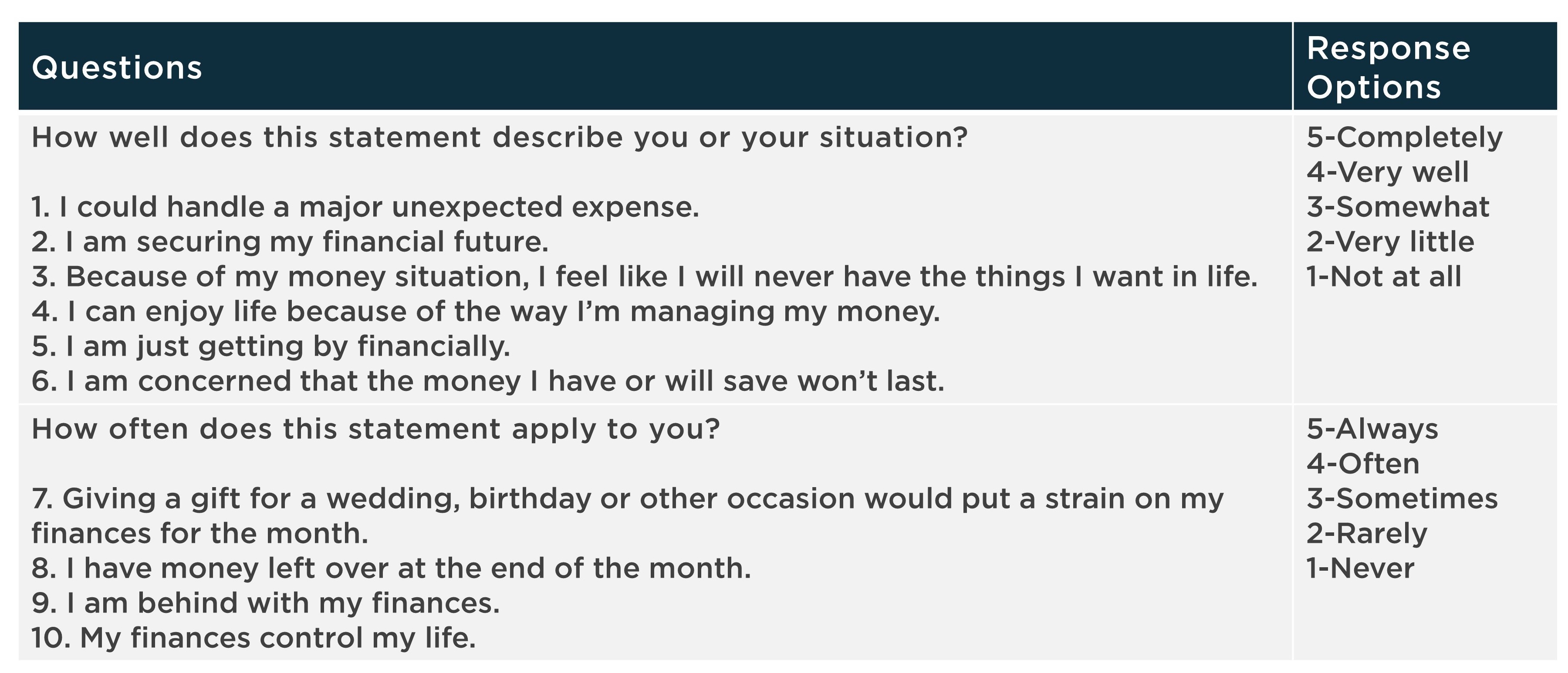
To measure the construct of financial well-being, CFPB created the Financial Well-Being Scale that consists of ten rating scale items. The items cover all four elements of the CFPB’s definition of financial well-being: control over finances, capacity to absorb a financial shock, being on track to meet financial goals, and having the financial freedom to enjoy life, using both positive and negative phrasing. Figure 1 shows a list of the items and their response options.

Figure 1: Items in the Financial Well-Being Scale (Source: Consumer Financial Protection Bureau)

The CFPB’s technical report on the Financial Well-Being (FWB) Scale indicates that the researchers tested several different models, including a unidimensional model, several multidimensional models defined a priori by substantive item content, and other models indicated by initial exploratory analyses that reflected methodological considerations (such as positive versus negative item wording). Although the instrument was supposed to measure financial well-being as a single (i.e., unidimensional) construct, the researchers found that the bi-factor model fit the data best, with a general factor related to the latent financial well-being construct and two additional factors associated with the polarity of the item (i.e., whether the item was phrased negatively or positively).

For demonstration purposes, we will assume that we do not have any priori hypothesis about the factorial structure (i.e., dimensionality) of the FWB Scale, or we believe that the construct of financial well-being may be unidimensional though we are not entirely sure at this point. Therefore, we will begin our analysis with an exploratory approach–Parallel Analysis–to evaluate the dimensionality of this scale. Once we get an idea of what the factor structure may look like, we will switch to confirmatory factor analysis (CFA) to verify the structure. The dataset for this example is “finance.csv”. This dataset consists of 3822 individuals’ responses to 10 items in the FWB Scale, demographic variables, and additional variables related to financial well-being. The finance dataset can be downloaded from finance.csv. In addition, the R codes for the analyses presented in this section are available in example2.R.

Exploratory Data Analysis

We will begin our analysis by conducting exploratory data analysis to check our dataset. We will first import finance.csv into R, save it as “finance”, and then review the variables in the dataset using descriptive statistics and visualizations.

finance <- read.csv("finance.csv", header = TRUE)

Using the head() function, we can now view the first 6 rows of the finance dataset:

head(finance)

  respondent_id   age gender              education                                     employment
1          7740 35-44   Male High school degree/GED Work full-time for an employer or the military
2         13699 35-44   Male Some college/Associate Work full-time for an employer or the military
3          7267 35-44   Male High school degree/GED                                        Refused
4          7375 25-34   Male High school degree/GED Work full-time for an employer or the military
5         10910 25-34   Male      Bachelor's degree Work full-time for an employer or the military
6         11079 35-44 Female      Bachelor's degree                                      Homemaker
      marital_status fwb1_1 fwb1_2 fwb1_3 fwb1_4 fwb1_5 fwb1_6 fwb2_1 fwb2_2 fwb2_3 fwb2_4 raise2000
1 Divorced/Separated      2      2      3      3      3      4      2      2      2      3         3
2 Divorced/Separated      3      3      3      3      3      3      3      3      3      3         4
3 Divorced/Separated      3      3      3      3      3      3      3      3      3      3         8
4            Married      3      3      3      3      3      3      3      3      3      3         2
5            Married      5      1      1      1      1      1      2      5      2      2         4
6            Married      1      3      2      3      3      3      3      2      1      4         4
  financial_knowledge debt_collector hardship_food hardship_doctor
1                   5              1             1               1
2                   5              0             1               1
3                  -1             -1             2               2
4                   4              8             2               2
5                   6              0             1               1
6                   5              0             1               1

The variables in the datasets are as follows:

respondent_id: Respondent ID
age: Age category
gender: Male or Female
education: Education level
employment: Employment status
marital_status: Marital status
fwb1_1 to fwb1_6: First six items with 1=Not at all to 5=Completely
fwb2_1 to fwb2_4: The last four items with 1=Never to 5=Always
raise2000: Confidence in ability to raise $2000 in 30 days
financial_knowledge: Overall financial knowledge (self-reported)
debt_collector: Contacted by a debt collector in past 12 months
hardship_food: Food didn’t last and didn’t have money to get more
hardship_doctor: Any household member couldn’t afford to see doctor or go to hospital

As we are going to use the responses in this example, let’s save it as a separate dataset and then use the describe function from the psych package to examine the dataset:

response <- finance %>%
  dplyr::select(dplyr::starts_with("fwb"))

psych::describe(response)

	vars	n	mean	sd	min	max	range	se
fwb1_1	1	3,822	2.89	1.24	-4	5	9	0.020
fwb1_2	2	3,822	3.08	1.12	-4	5	9	0.018
fwb1_3	3	3,822	2.68	1.20	-4	5	9	0.019
fwb1_4	4	3,822	3.14	1.05	-4	5	9	0.017
fwb1_5	5	3,822	2.86	1.25	-4	5	9	0.020
fwb1_6	6	3,822	3.24	1.14	-4	5	9	0.018
fwb2_1	7	3,822	2.48	1.20	-4	5	9	0.019
fwb2_2	8	3,822	3.27	1.27	-4	5	9	0.020
fwb2_3	9	3,822	2.21	1.15	-4	5	9	0.019
fwb2_4	10	3,822	2.82	1.14	-4	5	9	0.018

The summary above shows that the minimum response value for the scale items is -4. The codebook for this dataset shows that missing responses are coded as -1 and -4 in the dataset. So, we will have to change these values to NA.

# Recode missing items
response <- apply(response, # data to apply the function
                  2, # 1 to apply to each row; 2 to apply to each column
                  function(x) ifelse(x %in% c(-1, -4), NA, x)) %>%
  as.data.frame()

Now, we can review the cleaned dataset. First, we will review if the response options have been properly utilized in each item.

apply(response, 2, table)

  fwb1_1 fwb1_2 fwb1_3 fwb1_4 fwb1_5 fwb1_6 fwb2_1 fwb2_2 fwb2_3 fwb2_4
1    671    382    634    269    605    237    894    367   1214    459
2    670    633   1178    617    892    688   1202    691   1294   1078
3   1272   1441   1139   1559   1236   1467   1001   1086    780   1285
4    797    983    478    998    572    750    415    866    320    648
5    406    376    387    372    509    674    304    804    207    345

Next, we will visualize the data:

DataExplorer::introduce(response)

  rows columns discrete_columns continuous_columns all_missing_columns
1 3822      10                0                 10                   0
  total_missing_values complete_rows total_observations memory_usage
1                   68          3811              38220       155832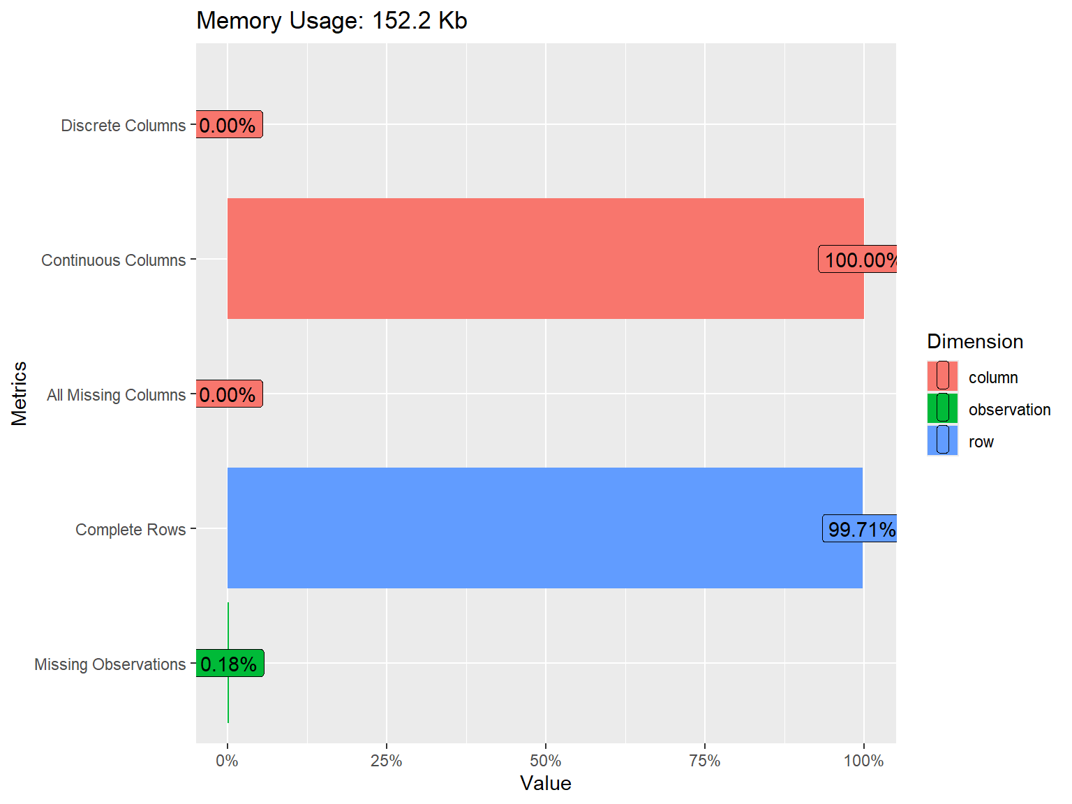

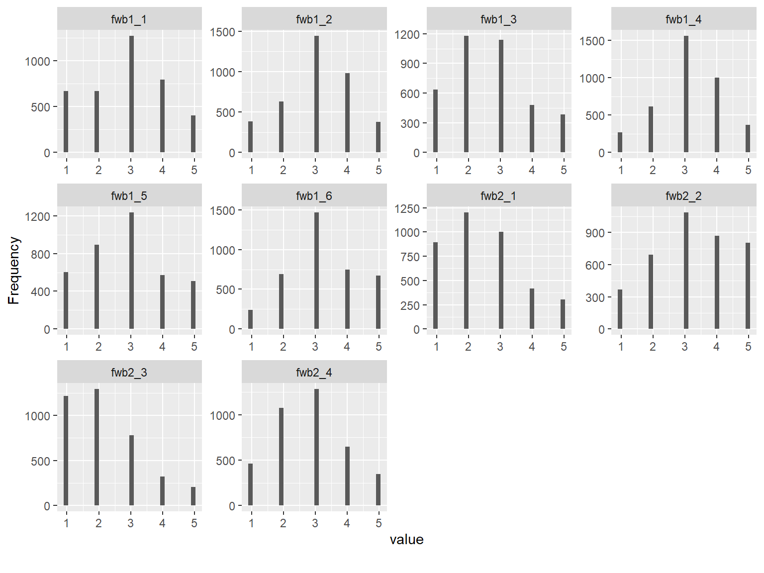
DataExplorer::plot_intro(response)

DataExplorer::plot_histogram(response)

The dataset consists of 3822 rows (i.e., respondents) and 10 variables (i.e., FWB Scale Items). The response options are distributed nicely across the items, although some items such as fwb2_3 have a skewed distribution. To better understand the relationships among the items, we will also check the correlations. Since the items are polytomously scored, we will compute the inter-item correlations among the items using the polychoric() function from psych and then extract “rho” (i.e., the correlation matrix of the items).

# Save the correlation matrix
cormat <- psych::polychoric(x = response)$rho

# Print the correlation matrix
print(cormat)

	fwb1_1	fwb1_2	fwb1_3	fwb1_4	fwb1_5	fwb1_6	fwb2_1	fwb2_2	fwb2_3	fwb2_4
fwb1_1	1.000	0.727	-0.528	0.729	-0.519	-0.488	-0.632	0.711	-0.556	-0.500
fwb1_2	0.727	1.000	-0.538	0.742	-0.436	-0.506	-0.564	0.647	-0.486	-0.458
fwb1_3	-0.528	-0.538	1.000	-0.552	0.601	0.654	0.637	-0.556	0.553	0.581
fwb1_4	0.729	0.742	-0.552	1.000	-0.451	-0.491	-0.574	0.672	-0.538	-0.499
fwb1_5	-0.519	-0.436	0.601	-0.451	1.000	0.522	0.574	-0.530	0.512	0.493
fwb1_6	-0.488	-0.506	0.654	-0.491	0.522	1.000	0.545	-0.504	0.469	0.545
fwb2_1	-0.632	-0.564	0.637	-0.574	0.574	0.545	1.000	-0.689	0.687	0.643
fwb2_2	0.711	0.647	-0.556	0.672	-0.530	-0.504	-0.689	1.000	-0.621	-0.532
fwb2_3	-0.556	-0.486	0.553	-0.538	0.512	0.469	0.687	-0.621	1.000	0.596
fwb2_4	-0.500	-0.458	0.581	-0.499	0.493	0.545	0.643	-0.532	0.596	1.000

The correlation matrix above shows negative correlations among the items due to positive/negative wording of the items in the scale. To put the items in the same direction, we will reverse-recode the negatively-worded items in the scale.

# First, let's save the original variable names
names_fwb <- colnames(response)

# Reverse code negatively-worded items 3,5,6,7,9, and 10
keys <- c(1,1,-1,1,-1,-1,-1,1,-1,-1)
response_final <- psych::reverse.code(keys, 
                                      items = response,
                                      mini = rep(1, 10),
                                      maxi = rep(5, 10))

# View the recoded dataset
head(response_final)

     fwb1_1 fwb1_2 fwb1_3- fwb1_4 fwb1_5- fwb1_6- fwb2_1- fwb2_2 fwb2_3-
[1,]      2      2       3      3       3       2       4      2       4
[2,]      3      3       3      3       3       3       3      3       3
[3,]      3      3       3      3       3       3       3      3       3
[4,]      3      3       3      3       3       3       3      3       3
[5,]      5      1       5      1       5       5       4      5       4
[6,]      1      3       4      3       3       3       3      2       5
     fwb2_4-
[1,]       3
[2,]       3
[3,]       3
[4,]       3
[5,]       4
[6,]       2

# Now let's change the names to the original names to avoid "-" added to the names
colnames(response_final) <- names_fwb

# Finally, recalculate the correlation matrix
cormat <- psych::polychoric(x = response_final)$rho

Next, we will check the associations among the items in the new dataset using a correlation matrix plot to confirm that the items are all positively correlated.

ggcorrplot::ggcorrplot(corr = cormat, # correlation matrix
                       type = "lower", # print only the lower part of the correlation matrix
                       hc.order = TRUE, # hierarchical clustering
                       show.diag = TRUE, # show the diagonal values of 1
                       lab = TRUE, # add correlation values as labels
                       lab_size = 3) # Size of the labels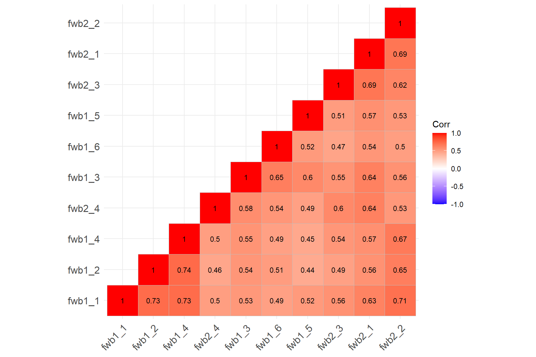

The correlation matrix plot confirms that all the items are now positively correlated with each other. We can begin to analyze the items. Note that if there is any item wording effect present in the data, reverse-coding the items would not necessarily fix the problem. We will see a good example of this situation in the following analyses.

Parallel Analysis

Parallel analysis compares the magnitude or size of eigenvalues generated from random data against the eigenvalues from the sample correlation matrix generated by the model. The main idea is that meaningful associations in the data should yield eigenvalues larger than would be expected by change.

parallel.test <- psych::fa.parallel(x = response_final, 
                                    fm="ml", # maximum likelihood
                                    fa="fa", # principal axis factor analysis
                                    cor="poly", # use polychoric correlations
                                    n.iter = 20, # number of iterations
                                    error.bars = TRUE)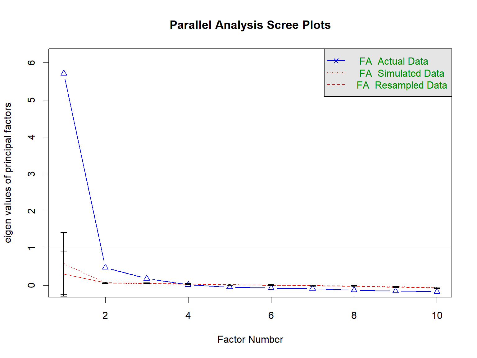

Parallel analysis suggests that the number of factors =  3  and the number of components =  NA

print(parallel.test)

Call: psych::fa.parallel(x = response_final, fm = "ml", fa = "fa", 
    n.iter = 20, error.bars = TRUE, cor = "poly")
Parallel analysis suggests that the number of factors =  3  and the number of components =  NA 

 Eigen Values of 

 eigen values of factors
 [1]  5.71  0.48  0.18  0.01 -0.05 -0.08 -0.09 -0.13 -0.15 -0.17

 eigen values of simulated factors
 [1]  0.59  0.06  0.04  0.03  0.02  0.00 -0.01 -0.03 -0.04 -0.06

 eigen values of components 
 [1] 6.13 0.91 0.63 0.52 0.38 0.34 0.32 0.28 0.25 0.24

 eigen values of simulated components
[1] NA

The results of our parallel analysis suggest that there are possibly three factors underlying the responses to the FWB Scale. We can increase the number of iterations and try again, though it is very like that the result will remain the same.

Confirmatory Factor Analysis

In CFA, the researcher must specify the expected relationships between indicators (i.e., observed variables) and latent factors. In other words, one must have an explicit account of what factor(s) underlie each item. In this example, we will evaluate two scenarios about the FCW Scale: two-factor structure (separate dimensions based on positive and negative wording), and a bi-factor structure with a general dimension and separate dimensions based on positive and negative wording.

We will use the lavaan package (Rosseel et al., 2023) (see https://lavaan.ugent.be/ for more information on the package) to estimate our CFA models. To understand how to set up a CFA model in lavaan, we can use the following table on the lavaan website (https://lavaan.ugent.be/tutorial/syntax1.html).

Formula Type	lavaan Operator	Meaning
Latent variable	=~	is measured by
Regression	~	is regressed on
Residual co(variance)	~~	is correlated with
Intercept	~1	intercept

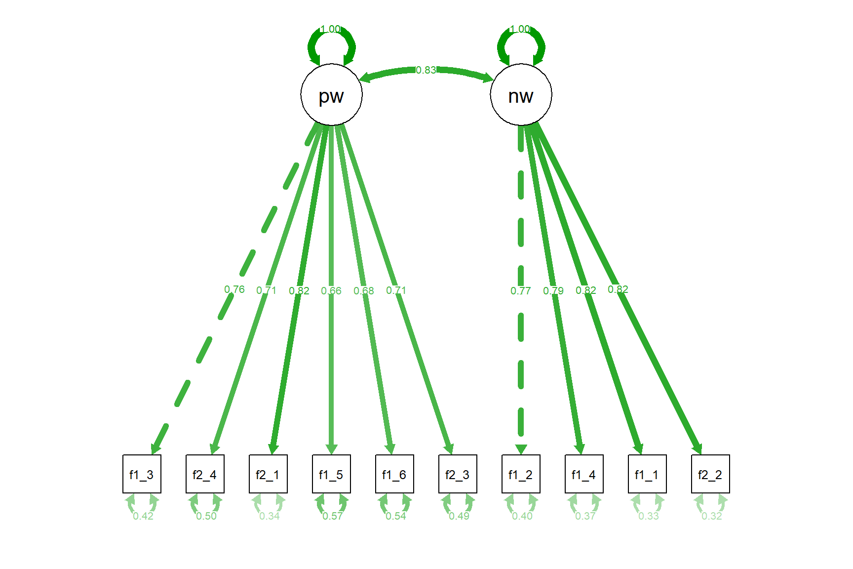
The format used in lavaan is fairly simple, and resembles a series of linear models, written over several lines. In the model below, there are two latent variables, pw and nw, referring to the positive wording and negative wording. The latent variable names are followed by =~ which means “is manifested by”, and then the observed variables are listed, separated by the “+” sign.

# Define a two-factor model
model.two <- '# Define factors
              pw =~ fwb1_3 + fwb2_4 + fwb2_1 + fwb1_5 + fwb1_6 + fwb2_3
              nw =~ fwb1_2 + fwb1_4 + fwb1_1 + fwb2_2
          
              # Variances and covariances
              pw ~~ pw
              nw ~~ nw
              pw ~~ nw'

Using the model above will give us factor loadings for the item, variances for the latent factors, and the covariance or correlation between the two factors we defined. Alternatively, we could use pw ~~ 0*nw to force orthogonal (uncorrelated) factors if our hypothesis about the underlying factor structure assumed uncorrelated factors. Also, this model will fix the factor loading for the first item associated with each factor to 1. We could free these items by fixing the variance of the factors to 1 to maintain the same degrees of freedom.

model.two <- '# Define factors
              pw =~ NA*fwb1_3 + fwb2_4 + fwb2_1 + fwb1_5 + fwb1_6 + fwb2_3
              nw =~ NA*fwb1_2 + fwb1_4 + fwb1_1 + fwb2_2
          
              # Variances and covariances
              pw ~~ 1*pw
              nw ~~ 1*nw
              pw ~~ nw'

Once a model is defined properly, it can be used within the cfa function to fit the model to the data. In the following example, we will use estimator = "WLSMV" because our items are polytomous and this particular estimator is designed to deal with ordinal or categorical variables that may not necessarily have a normal distribution.

cfa.wlsmv <- lavaan::cfa(model.two, data = response_final, estimator = "WLSMV")

Once the model has been fitted, the summary() function provides a nice summary of the fitted model. To better interpret the factor loadings, we request the standardized solutions by using standardized=TRUE.

summary(cfa.wlsmv, fit.measures=TRUE, standardized=TRUE)

lavaan 0.6.17 ended normally after 30 iterations

  Estimator                                       DWLS
  Optimization method                           NLMINB
  Number of model parameters                        21

                                                  Used       Total
  Number of observations                          3811        3822

Model Test User Model:
                                              Standard      Scaled
  Test Statistic                               164.740     602.565
  Degrees of freedom                                34          34
  P-value (Chi-square)                           0.000       0.000
  Scaling correction factor                                  0.276
  Shift parameter                                            5.125
    simple second-order correction                                

Model Test Baseline Model:

  Test statistic                             38152.934   13355.485
  Degrees of freedom                                45          45
  P-value                                        0.000       0.000
  Scaling correction factor                                  2.863

User Model versus Baseline Model:

  Comparative Fit Index (CFI)                    0.997       0.957
  Tucker-Lewis Index (TLI)                       0.995       0.943
                                                                  
  Robust Comparative Fit Index (CFI)                         0.996
  Robust Tucker-Lewis Index (TLI)                            0.995

Root Mean Square Error of Approximation:

  RMSEA                                          0.032       0.066
  90 Percent confidence interval - lower         0.027       0.062
  90 Percent confidence interval - upper         0.037       0.071
  P-value H_0: RMSEA <= 0.050                    1.000       0.000
  P-value H_0: RMSEA >= 0.080                    0.000       0.000
                                                                  
  Robust RMSEA                                               0.035
  90 Percent confidence interval - lower                     0.032
  90 Percent confidence interval - upper                     0.037
  P-value H_0: Robust RMSEA <= 0.050                         1.000
  P-value H_0: Robust RMSEA >= 0.080                         0.000

Standardized Root Mean Square Residual:

  SRMR                                           0.031       0.031

Parameter Estimates:

  Standard errors                           Robust.sem
  Information                                 Expected
  Information saturated (h1) model        Unstructured

Latent Variables:
                   Estimate  Std.Err  z-value  P(>|z|)   Std.lv  Std.all
  pw =~                                                                 
    fwb1_3            1.000                               0.899    0.759
    fwb2_4            0.882    0.022   39.604    0.000    0.793    0.705
    fwb2_1            1.078    0.023   46.925    0.000    0.970    0.815
    fwb1_5            0.904    0.028   32.685    0.000    0.813    0.656
    fwb1_6            0.849    0.020   41.722    0.000    0.763    0.677
    fwb2_3            0.903    0.024   38.403    0.000    0.812    0.712
  nw =~                                                                 
    fwb1_2            1.000                               0.850    0.773
    fwb1_4            0.967    0.019   52.182    0.000    0.822    0.794
    fwb1_1            1.184    0.022   54.041    0.000    1.007    0.821
    fwb2_2            1.211    0.024   50.816    0.000    1.030    0.824

Covariances:
                   Estimate  Std.Err  z-value  P(>|z|)   Std.lv  Std.all
  pw ~~                                                                 
    nw                0.636    0.021   30.139    0.000    0.832    0.832

Variances:
                   Estimate  Std.Err  z-value  P(>|z|)   Std.lv  Std.all
    pw                0.809    0.030   26.932    0.000    1.000    1.000
    nw                0.723    0.025   29.047    0.000    1.000    1.000
   .fwb1_3            0.596    0.022   27.211    0.000    0.596    0.424
   .fwb2_4            0.637    0.022   28.861    0.000    0.637    0.503
   .fwb2_1            0.474    0.019   25.247    0.000    0.474    0.335
   .fwb1_5            0.874    0.032   26.966    0.000    0.874    0.569
   .fwb1_6            0.690    0.023   29.956    0.000    0.690    0.542
   .fwb2_3            0.640    0.021   31.175    0.000    0.640    0.493
   .fwb1_2            0.488    0.016   29.619    0.000    0.488    0.403
   .fwb1_4            0.397    0.015   25.735    0.000    0.397    0.370
   .fwb1_1            0.490    0.021   23.881    0.000    0.490    0.326
   .fwb2_2            0.500    0.022   23.052    0.000    0.500    0.320

To evaluate the model fit, we will use Hu & Bentler (1999)’s guidelines for model fit indices: (1) Comparative fit index (CFI) > .95; Tucker-Lewis index (TLI) > .95; and root mean square error of approximation (RMSEA) < .06. The output shows that the model fits the data very nicely!

In the output, the columns, Std.lv and Std.all, correspond to slightly different solutions. The Std.all solution standardizes the factor loadings by the standard deviation of both the predictor (the factor, X) and the outcome (the item, Y). In the variance standardization method Std.lv, we only standardize by the predictor (the factor, X). Comparing the two solutions, the loadings and variance of the factors are different but the residual variances are the same.

Using the semPaths function from the semPlot package, we can also visualize the model by creating a path diagram:

semPlot::semPaths(cfa.wlsmv, "std") # "std" gives standardized loadings

Let’s also run the same model with robust maximum likelihood (known as MLR estimator) and check out the results.

cfa.mlr <- lavaan::cfa(model.two, data = response_final, estimator = "MLR")
summary(cfa.mlr, fit.measures=TRUE, standardized=TRUE)

lavaan 0.6.17 ended normally after 25 iterations

  Estimator                                         ML
  Optimization method                           NLMINB
  Number of model parameters                        21

                                                  Used       Total
  Number of observations                          3811        3822

Model Test User Model:
                                              Standard      Scaled
  Test Statistic                               827.665     650.309
  Degrees of freedom                                34          34
  P-value (Chi-square)                           0.000       0.000
  Scaling correction factor                                  1.273
    Yuan-Bentler correction (Mplus variant)                       

Model Test Baseline Model:

  Test statistic                             20848.665   14266.368
  Degrees of freedom                                45          45
  P-value                                        0.000       0.000
  Scaling correction factor                                  1.461

User Model versus Baseline Model:

  Comparative Fit Index (CFI)                    0.962       0.957
  Tucker-Lewis Index (TLI)                       0.950       0.943
                                                                  
  Robust Comparative Fit Index (CFI)                         0.962
  Robust Tucker-Lewis Index (TLI)                            0.950

Loglikelihood and Information Criteria:

  Loglikelihood user model (H0)             -49717.248  -49717.248
  Scaling correction factor                                  1.402
      for the MLR correction                                      
  Loglikelihood unrestricted model (H1)     -49303.416  -49303.416
  Scaling correction factor                                  1.322
      for the MLR correction                                      
                                                                  
  Akaike (AIC)                               99476.497   99476.497
  Bayesian (BIC)                             99607.656   99607.656
  Sample-size adjusted Bayesian (SABIC)      99540.927   99540.927

Root Mean Square Error of Approximation:

  RMSEA                                          0.078       0.069
  90 Percent confidence interval - lower         0.074       0.065
  90 Percent confidence interval - upper         0.083       0.073
  P-value H_0: RMSEA <= 0.050                    0.000       0.000
  P-value H_0: RMSEA >= 0.080                    0.274       0.000
                                                                  
  Robust RMSEA                                               0.078
  90 Percent confidence interval - lower                     0.073
  90 Percent confidence interval - upper                     0.083
  P-value H_0: Robust RMSEA <= 0.050                         0.000
  P-value H_0: Robust RMSEA >= 0.080                         0.251

Standardized Root Mean Square Residual:

  SRMR                                           0.033       0.033

Parameter Estimates:

  Standard errors                             Sandwich
  Information bread                           Observed
  Observed information based on                Hessian

Latent Variables:
                   Estimate  Std.Err  z-value  P(>|z|)   Std.lv  Std.all
  pw =~                                                                 
    fwb1_3            1.000                               0.899    0.758
    fwb2_4            0.894    0.022   40.068    0.000    0.804    0.715
    fwb2_1            1.068    0.024   44.145    0.000    0.960    0.808
    fwb1_5            0.904    0.026   34.175    0.000    0.813    0.656
    fwb1_6            0.848    0.019   44.935    0.000    0.762    0.676
    fwb2_3            0.902    0.025   36.262    0.000    0.811    0.712
  nw =~                                                                 
    fwb1_2            1.000                               0.873    0.793
    fwb1_4            0.957    0.017   56.853    0.000    0.835    0.806
    fwb1_1            1.165    0.020   56.982    0.000    1.017    0.830
    fwb2_2            1.132    0.024   48.177    0.000    0.988    0.791

Covariances:
                   Estimate  Std.Err  z-value  P(>|z|)   Std.lv  Std.all
  pw ~~                                                                 
    nw                0.651    0.021   31.578    0.000    0.829    0.829

Variances:
                   Estimate  Std.Err  z-value  P(>|z|)   Std.lv  Std.all
    pw                0.808    0.030   26.549    0.000    1.000    1.000
    nw                0.762    0.025   29.939    0.000    1.000    1.000
   .fwb1_3            0.597    0.022   26.857    0.000    0.597    0.425
   .fwb2_4            0.619    0.021   29.059    0.000    0.619    0.489
   .fwb2_1            0.491    0.019   25.906    0.000    0.491    0.348
   .fwb1_5            0.873    0.032   27.445    0.000    0.873    0.569
   .fwb1_6            0.691    0.023   30.000    0.000    0.691    0.543
   .fwb2_3            0.642    0.021   30.895    0.000    0.642    0.494
   .fwb1_2            0.449    0.016   27.664    0.000    0.449    0.371
   .fwb1_4            0.375    0.015   25.055    0.000    0.375    0.350
   .fwb1_1            0.468    0.020   23.986    0.000    0.468    0.312
   .fwb2_2            0.584    0.021   27.271    0.000    0.584    0.374

The results show that the estimated values for factor loadings, residuals, correlation between the factors have changed slightly when we used the MLR estimator. Compared with the WLSMV solution, the model fit indices are slightly worse, indicating that WLSMV provided a better solution. This is not necessarily surprising given that the items in the FWB scale are all polytomous.

In addition to the two-factor solution, we will also try the bi-factor model. We can achieve this either manually setting up the model with uncorrelated factors or using orthogonal=TRUE in the cfa function. We will use the easy way to set up our model. std.lv=TRUE is also a shortcut to get the factor variances fixed to 1 while getting free estimates of factor loadings for all items.

bi.model <- '# Define factors
             g =~ fwb1_3 + fwb2_4 + fwb2_1 + fwb1_5 + fwb1_6 + fwb2_3 + fwb1_2 + fwb1_4 + fwb1_1 + fwb2_2
             pw =~ fwb1_3 + fwb2_4 + fwb2_1 + fwb1_5 + fwb1_6 + fwb2_3
             nw =~ fwb1_2 + fwb1_4 + fwb1_1 + fwb2_2'

bifactor.wlsmv <- cfa(bi.model, data=response_final, estimator = "WLSMV", 
                      orthogonal=TRUE, std.lv=TRUE)
summary(bifactor.wlsmv, fit.measures=TRUE, standardized=TRUE)

lavaan 0.6.17 ended normally after 69 iterations

  Estimator                                       DWLS
  Optimization method                           NLMINB
  Number of model parameters                        30

                                                  Used       Total
  Number of observations                          3811        3822

Model Test User Model:
                                              Standard      Scaled
  Test Statistic                                41.084     194.922
  Degrees of freedom                                25          25
  P-value (Chi-square)                           0.022       0.000
  Scaling correction factor                                  0.213
  Shift parameter                                            2.283
    simple second-order correction                                

Model Test Baseline Model:

  Test statistic                             38152.934   13355.485
  Degrees of freedom                                45          45
  P-value                                        0.000       0.000
  Scaling correction factor                                  2.863

User Model versus Baseline Model:

  Comparative Fit Index (CFI)                    1.000       0.987
  Tucker-Lewis Index (TLI)                       0.999       0.977
                                                                  
  Robust Comparative Fit Index (CFI)                         0.999
  Robust Tucker-Lewis Index (TLI)                            0.998

Root Mean Square Error of Approximation:

  RMSEA                                          0.013       0.042
  90 Percent confidence interval - lower         0.005       0.037
  90 Percent confidence interval - upper         0.020       0.048
  P-value H_0: RMSEA <= 0.050                    1.000       0.989
  P-value H_0: RMSEA >= 0.080                    0.000       0.000
                                                                  
  Robust RMSEA                                               0.020
  90 Percent confidence interval - lower                     0.017
  90 Percent confidence interval - upper                     0.022
  P-value H_0: Robust RMSEA <= 0.050                         1.000
  P-value H_0: Robust RMSEA >= 0.080                         0.000

Standardized Root Mean Square Residual:

  SRMR                                           0.016       0.016

Parameter Estimates:

  Standard errors                           Robust.sem
  Information                                 Expected
  Information saturated (h1) model        Unstructured

Latent Variables:
                   Estimate  Std.Err  z-value  P(>|z|)   Std.lv  Std.all
  g =~                                                                  
    fwb1_3            0.883    0.019   47.545    0.000    0.883    0.745
    fwb2_4            0.789    0.017   46.473    0.000    0.789    0.701
    fwb2_1            0.994    0.016   61.613    0.000    0.994    0.836
    fwb1_5            0.799    0.022   35.622    0.000    0.799    0.645
    fwb1_6            0.750    0.019   38.577    0.000    0.750    0.665
    fwb2_3            0.838    0.018   45.852    0.000    0.838    0.736
    fwb1_2            0.684    0.018   37.475    0.000    0.684    0.622
    fwb1_4            0.669    0.018   38.133    0.000    0.669    0.645
    fwb1_1            0.828    0.019   44.188    0.000    0.828    0.675
    fwb2_2            0.899    0.018   50.125    0.000    0.899    0.720
  pw =~                                                                 
    fwb1_3            0.344    0.037    9.383    0.000    0.344    0.291
    fwb2_4            0.048    0.029    1.636    0.102    0.048    0.043
    fwb2_1           -0.166    0.038   -4.372    0.000   -0.166   -0.139
    fwb1_5            0.196    0.036    5.508    0.000    0.196    0.158
    fwb1_6            0.416    0.037   11.100    0.000    0.416    0.369
    fwb2_3           -0.197    0.031   -6.297    0.000   -0.197   -0.172
  nw =~                                                                 
    fwb1_2            0.578    0.022   25.766    0.000    0.578    0.525
    fwb1_4            0.522    0.021   24.723    0.000    0.522    0.504
    fwb1_1            0.591    0.024   24.567    0.000    0.591    0.482
    fwb2_2            0.388    0.026   14.912    0.000    0.388    0.310

Covariances:
                   Estimate  Std.Err  z-value  P(>|z|)   Std.lv  Std.all
  g ~~                                                                  
    pw                0.000                               0.000    0.000
    nw                0.000                               0.000    0.000
  pw ~~                                                                 
    nw                0.000                               0.000    0.000

Variances:
                   Estimate  Std.Err  z-value  P(>|z|)   Std.lv  Std.all
   .fwb1_3            0.507    0.027   19.105    0.000    0.507    0.361
   .fwb2_4            0.641    0.022   29.182    0.000    0.641    0.506
   .fwb2_1            0.398    0.026   15.129    0.000    0.398    0.281
   .fwb1_5            0.857    0.032   26.963    0.000    0.857    0.559
   .fwb1_6            0.537    0.031   17.492    0.000    0.537    0.422
   .fwb2_3            0.558    0.025   22.324    0.000    0.558    0.429
   .fwb1_2            0.409    0.018   22.409    0.000    0.409    0.338
   .fwb1_4            0.354    0.016   22.204    0.000    0.354    0.330
   .fwb1_1            0.468    0.021   22.428    0.000    0.468    0.311
   .fwb2_2            0.603    0.020   30.476    0.000    0.603    0.386
    g                 1.000                               1.000    1.000
    pw                1.000                               1.000    1.000
    nw                1.000                               1.000    1.000

Let’s also see the results visually:

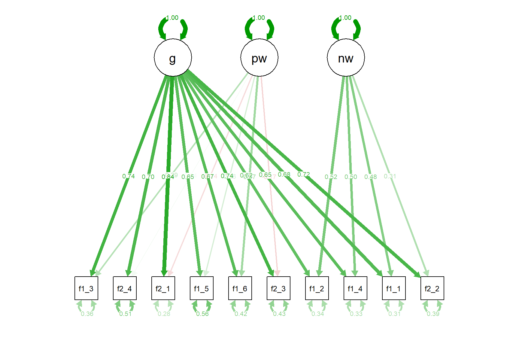
semPlot::semPaths(bifactor.wlsmv, "std") # "std" gives standardized loadings

The bi-factor model also seems to fit the data nicely (even slightly better than the two-factor model) but we see that some factor loadings are negative. This is probably the strength of the general (g) factor we defined. This factor absorbs most of the variance in the items, leaving only small variance to be explained by the pw and nw factors. At this point, we may believe that there is an overall factor of financial well-being but it is hard to extract in a unidimensional model due to item wording effects. Using the bi-factor model could possibly partial out the variance due to item wording while accounting for a large amount of variance available in the items.

We can run a quick model comparison using the anova function.

anova(cfa.wlsmv, bifactor.wlsmv)


Scaled Chi-Squared Difference Test (method = "satorra.2000")

lavaan NOTE:
    The "Chisq" column contains standard test statistics, not the
    robust test that should be reported per model. A robust difference
    test is a function of two standard (not robust) statistics.
 
               Df AIC BIC Chisq Chisq diff Df diff Pr(>Chisq)    
bifactor.wlsmv 25          41.1                                  
cfa.wlsmv      34         164.7        322       9     <2e-16 ***
---
Signif. codes:  0 '***' 0.001 '**' 0.01 '*' 0.05 '.' 0.1 ' ' 1

2.1.0.1 Principal Component Analysis (PCA)

We will finish this example with a small demonstration of how principal component analysis works. This time, we will use the last five variables in the finance dataset:

raise2000: Confidence in ability to raise $2000 in 30 days (1 to 4, higher values indicate higher confidence)
financial_knowledge: Overall financial knowledge (1 to 7, higher alues indicate higher knowledge)
debt_collector: Contacted by a debt collector in past 12 months (1=yes, 0=no)
hardship_food: Food didn’t last and didn’t have money to get more (1=never, 2=sometimes, 3=often)
hardship_doctor: Any household member couldn’t afford to see doctor or go to hospital (1=never, 2=sometimes, 3=often)

Our goal is to reduce the number of these variables through PCA (rather than creating a latent variable based on these variables). After creating a separate dataset with these variables, we will deal with missing values. For each variable, -1 refers to “Refused to respond” and 8 refers to “Not sure”. So, we will recode these values as NA.

# Select the variables of interest
data <- finance %>%
  dplyr::select(raise2000, financial_knowledge, debt_collector, 
                hardship_food, hardship_doctor)

# Recode missing items
data <- apply(data, # data to apply the function
              2, # 1 to apply to each row; 2 to apply to each column
              function(x) ifelse(x %in% c(-1, 8), NA, x)) %>%
  as.data.frame()

Next, we will use the principal function to perform PCA and extract one component.

pca_results1 <- psych::principal(
  r = data, 
  nfactors = 1, # Number of components to extract
  rotate="varimax",
  cor = "mixed" # for a mixture of tetrachorics, polychorics, and so on
)

print(pca_results1)

Principal Components Analysis
Call: psych::principal(r = data, nfactors = 1, rotate = "varimax", 
    cor = "mixed")
Standardized loadings (pattern matrix) based upon correlation matrix
                      PC1   h2   u2 com
raise2000           -0.87 0.75 0.25   1
financial_knowledge -0.47 0.22 0.78   1
debt_collector       0.77 0.59 0.41   1
hardship_food        0.88 0.78 0.22   1
hardship_doctor      0.80 0.64 0.36   1

                PC1
SS loadings    2.98
Proportion Var 0.60

Mean item complexity =  1
Test of the hypothesis that 1 component is sufficient.

The root mean square of the residuals (RMSR) is  0.11 
 with the empirical chi square  911  with prob <  1.1e-194 

Fit based upon off diagonal values = 0.95

The output shows that one component explains 60% of the total variance. Now, let’s also try two components and see if this increases the amount of explained variance:

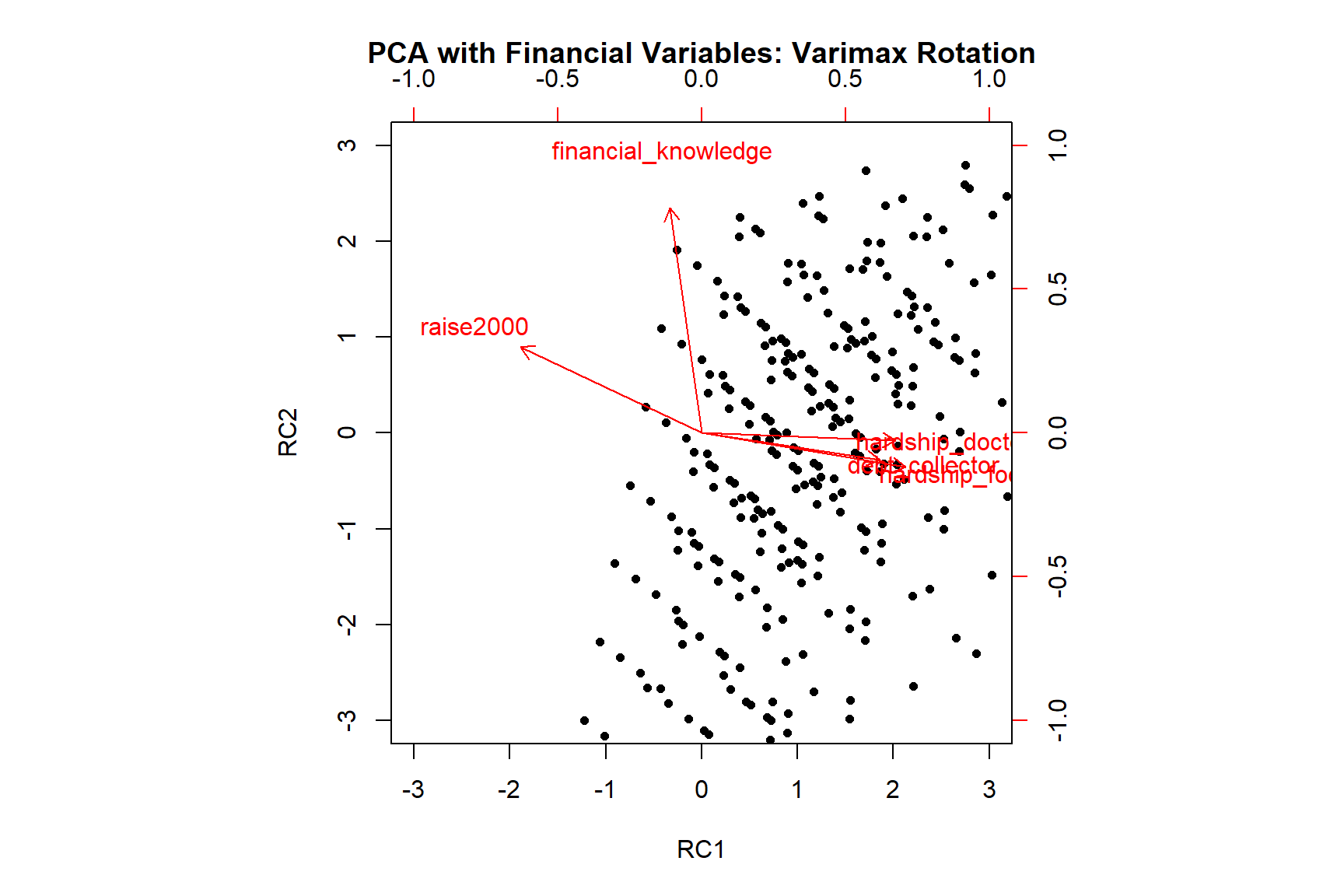
pca_results2a <- psych::principal(
  r = data, 
  nfactors = 2, 
  rotate="varimax",
  cor = "mixed"
)

print(pca_results2a)

Principal Components Analysis
Call: psych::principal(r = data, nfactors = 2, rotate = "varimax", 
    cor = "mixed")
Standardized loadings (pattern matrix) based upon correlation matrix
                      RC1   RC2   h2    u2 com
raise2000           -0.79  0.37 0.76 0.239 1.4
financial_knowledge -0.14  0.98 0.97 0.026 1.0
debt_collector       0.77 -0.12 0.61 0.387 1.0
hardship_food        0.89 -0.15 0.81 0.192 1.1
hardship_doctor      0.84 -0.03 0.71 0.290 1.0

                       RC1  RC2
SS loadings           2.74 1.13
Proportion Var        0.55 0.23
Cumulative Var        0.55 0.77
Proportion Explained  0.71 0.29
Cumulative Proportion 0.71 1.00

Mean item complexity =  1.1
Test of the hypothesis that 2 components are sufficient.

The root mean square of the residuals (RMSR) is  0.09 
 with the empirical chi square  573  with prob <  1.5e-126 

Fit based upon off diagonal values = 0.97

The two components seem to explain almost 77% of the total variance. This is great because now we can use these two components instead of all five variables if we want to include them in a predictive model (leading to higher model parsimony). Let’s also see the plot for this solution:

biplot(pca_results2a,
       main = "PCA with Financial Variables: Varimax Rotation")

Let’s also try to estimate the same model with oblique rotation.

pca_results2b <- psych::principal(
  r = data, 
  nfactors = 2, 
  rotate="promax",
  cor = "mixed"
)

print(pca_results2b)

Principal Components Analysis
Call: psych::principal(r = data, nfactors = 2, rotate = "promax", cor = "mixed")
Standardized loadings (pattern matrix) based upon correlation matrix
                      RC1  RC2   h2    u2 com
raise2000           -0.77 0.23 0.76 0.239 1.2
financial_knowledge  0.02 0.99 0.97 0.026 1.0
debt_collector       0.79 0.03 0.61 0.387 1.0
hardship_food        0.91 0.02 0.81 0.192 1.0
hardship_doctor      0.88 0.13 0.71 0.290 1.0

                       RC1  RC2
SS loadings           2.81 1.06
Proportion Var        0.56 0.21
Cumulative Var        0.56 0.77
Proportion Explained  0.73 0.27
Cumulative Proportion 0.73 1.00

 With component correlations of 
      RC1   RC2
RC1  1.00 -0.34
RC2 -0.34  1.00

Mean item complexity =  1
Test of the hypothesis that 2 components are sufficient.

The root mean square of the residuals (RMSR) is  0.09 
 with the empirical chi square  573  with prob <  1.5e-126 

Fit based upon off diagonal values = 0.97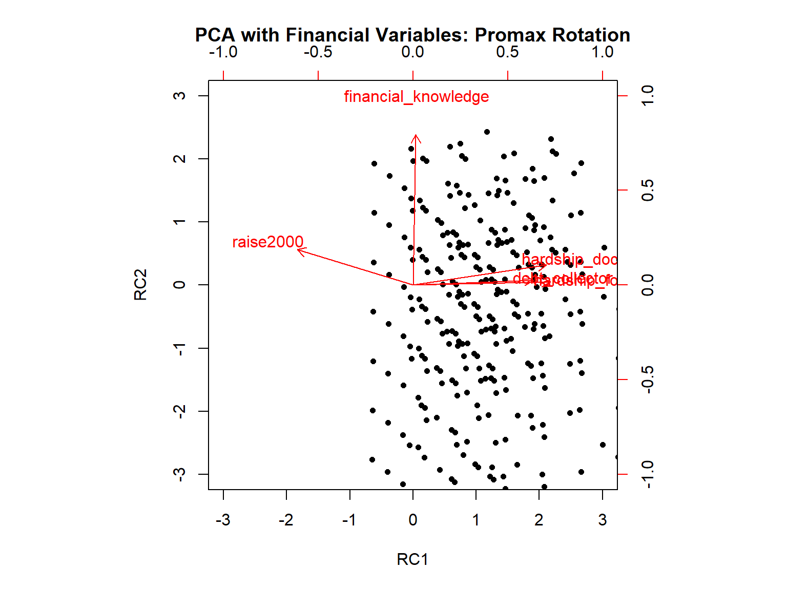

biplot(pca_results2b,
       main = "PCA with Financial Variables: Promax Rotation")

Exercises

Fit the two-factor CFA model to the data by forcing the correlation between the factors to be zero and compare the model fit to that of the correlated model we estimated earlier using the anova function.
Use the following model to fit a second-order (i.e., higher-order) model where the pw and nw factors define a higher-order factor of g (i.e., general factor). Note that there is no perfect way to specify a second-order factor when there are only two first-order factors. However, for the sake of our demonstration, we will give it a try and check its model it.

so.model <- '# Define factors
             pw =~ fwb1_3 + fwb2_4 + fwb2_1 + fwb1_5 + fwb1_6 + fwb2_3
             nw =~ fwb1_2 + fwb1_4 + fwb1_1 + fwb2_2
             g =~ 1*pw + 1*nw
             g ~~ g'

Nieto et al. (2021) show that there is an alternative way to model item wording effects in psychological instruments–the random intercept item factor analysis (RIIFA) model. In the RIIFA model introduced by Maydeu-Olivares & Coffman (2006), the researcher defines a factor associated with all items and an additional “wording” factor. This additional factor is also associated with all items. Its factor loadings are fixed to 1 but its variance is estimated (see Figure 1, Step 3 in Nieto et al. (2021)). Fit the RIIFA model to the FWB scale and evaluate the model fit. For this model, you will use the response dataset instead of response_final.

2.2 Psychometric Network Analysis

To be posted here…

References

Chalmers, P. (2023). Mirt: Multidimensional item response theory. https://github.com/philchalmers/mirt

Condon, D. M., & Revelle, W. (2014). The international cognitive ability resource: Development and initial validation of a public-domain measure. Intelligence, 43, 52–64.

Cui, B. (2020). DataExplorer: Automate data exploration and treatment. http://boxuancui.github.io/DataExplorer/

Hu, L., & Bentler, P. M. (1999). Cutoff criteria for fit indexes in covariance structure analysis: Conventional criteria versus new alternatives. Structural Equation Modeling: A Multidisciplinary Journal, 6(1), 1–55.

Maydeu-Olivares, A., & Coffman, D. L. (2006). Random intercept item factor analysis. Psychological Methods, 11(4), 344.

Revelle, W. (2022). Psych: Procedures for psychological, psychometric, and personality research. https://personality-project.org/r/psych/

Revelle, W., Wilt, J., & Rosenthal, A. (2010). Individual differences in cognition: New methods for examining the personality-cognition link. In Handbook of individual differences in cognition (pp. 27–49). Springer.

Ripley, B. (2023). MASS: Support functions and datasets for venables and ripley’s MASS. http://www.stats.ox.ac.uk/pub/MASS4/

Rosseel, Y., Jorgensen, T. D., & De Wilde, L. (2023). Lavaan: Latent variable analysis. https://lavaan.ugent.be