8 Supervised Machine Learning - Part II
8.1 Support Vector Machines
The support vector machine (SVM) is a family of related techniques developed in the 80s in computer science. They can be used in either a classification or a regression framework, but are principally known for/applied to classification (of which they are considered one of the best classification techniques because of their flexibility). Following James et al. (2013), we will make the distinction here between maximal margin classifiers (basically a support vector classifier with a cost parameter of 0 and a separating hyperplane), support vector classifiers (or an SVM with a linear kernel), and support vector machines (which employ non-linear kernels).
8.1.1 Maximal Margin Classifier
8.1.1.1 Hyperplane
The concept of a hyperplane is a critical concept in SVM, therefore, we need to understand what exactly a hyperplane is to understand SVM. A hyperplane is a subspace whose dimension is one less than that of the ambient space. Specifically, in a p-dimensional space, a hyperplane is a flat affline subspace of dimensional p - 1, where affline refers to the fact that the subspace need not pass through the origin.
We define a hyperplane as
\[ \beta_0 + \beta_1X_1 + \beta_2X_2 + \dots + \beta_pX_p = 0 \]
Where \(X_1, X_2, ..., X_p\) are predictors (or features). Therefore, for any observation of \(X = (X_1, X_2, \dots, X_p)^T\) that satisfies the above equation, the observation falls directly onto the hyperplane. However, a value of \(X\) does not need to fall onto the hyperplane, but could fall on either side of the hyperplane such that either
\[ \beta_0 + \beta_1X_1 + \beta_2X_2 + \cdots + \beta_pX_p > 0 \]
or
\[ \beta_0 + \beta_1X_1 + \beta_2X_2 + \cdots + \beta_pX_p < 0 \]
occurs. In that situation, the value of \(X\) lies on one of the two sides of the hyperplane and the hyperplane acts to split the p-dimensional space into two halves.
Figure 8.1 shows the hyperplane \(.5 + 1X_1 + -4X_2 = 0\). If we plug a value of \(X_1\) and \(X_2\) into this equation, we know based on the sign alone if the points falls on one side of the hyperplane or if it falls directly onto the hyperplane. In Figure 8.1 all the points in the red region will have negative signs (i.e., if we plug in the values of \(X_1\) and \(X_2\) into the above equation the sign will be negative), while all the points in the blue region would be positive, whereas any points that would have no sign are represented by the black line (the hyperplane).
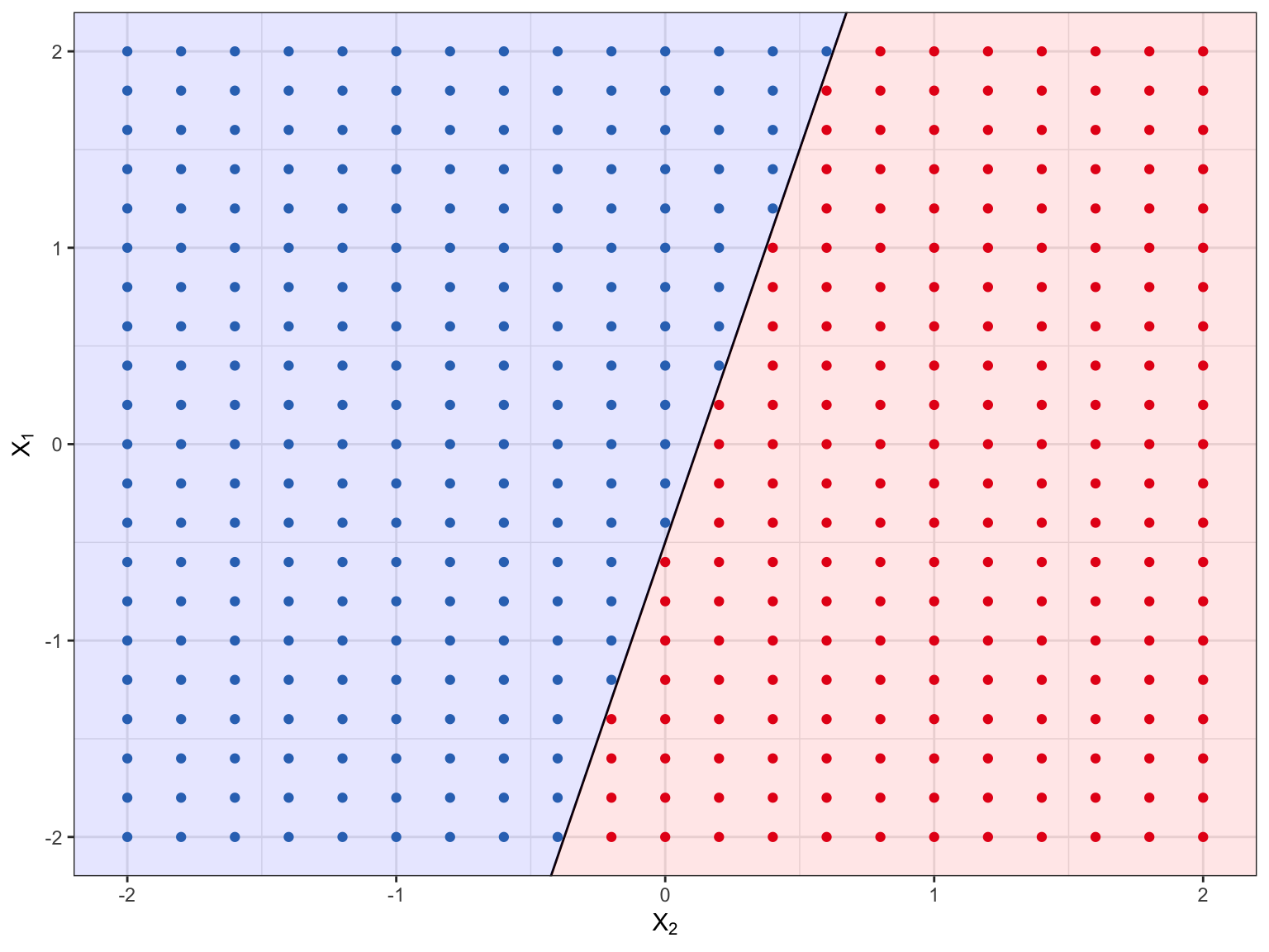
Figure 8.1: The hyperplane, \(.5 + 1X_1 + -4X_2 = 0\), is black line, the red points occur in the region where \(.5 + 1X_1 + -4X_2 > 0\), while the blue points occur in the region where \(.5 + 1X_1 + -4X_2 < 0\).
Wee can apply this idea of a hyperplane to classifying observations. We learned earlier how it important it is when applying machine learning techniques to split our data into training and testing data sets to avoid overfitting. We can split our n + m by p matrix of observations into an n by p \(\mathbf{X}\) matrix of training observations, which fall into one of two classes for \(Y = y_1, .., y_n\) where \(Y_i \in {-1, 1}\) and an m by p matrix \(\mathbf{X^*}\) of testing observations. Using just the training data, our goal is develop a model that will correctly classify our testing data using just a hyperplane and we will do this by creating a separating hyperplane (a hyperplane that will separate our classes).
Let’s assume we have the training data in Figure 8.2 and that the blue points correspond to one class (labelled as \(y = 1\)) and the red points correspond to the other class (\(y = -1\)). The separating hyper plane has the property that:
\[ \beta_0 + \beta_1x_{i1} + \beta_2x_{i2} + \dots + \beta_px_{p1} > 0 \quad \text{if} \quad y_i = 1 \] and \[ \beta_0 + \beta_1x_{i1} + \beta_2x_{i2} + \dots + \beta_px_{p1} < 0 \quad \text{if} \quad y_i = -1 \] Or more succintly, \[ y_i(\beta_0 + \beta_1x_{i1} + \beta_2x_{i2} + \dots + \beta_px_{p1}) > 0 \]
Ideally, we would create a hyperplane that perfectly separates the classes based on \(X_1\) and \(X_2\). However, as Figure 8.2 makes clear, we can create many separating hyperplanes of which 3 of these are shown. In fact, it’s often the case that an infinite number of separating hyperplanes could be created when the classes are perfectly separable. What we need to do is to develop some kind of a criterion for selecting one of the many separating hyperplanes.
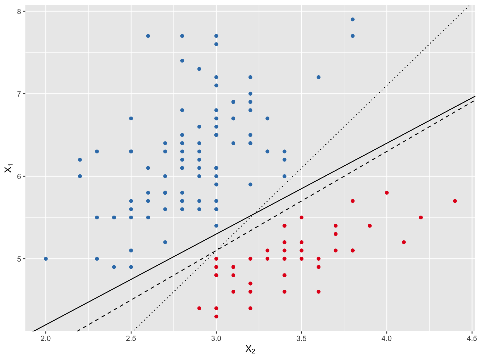
Figure 8.2: Candidate hyperplanes to separate the two classes.
For any given hyperplane, we have two pieces of information available for each observation: 1) the side of the hyperplane it lies on (represented by its sign) and 2) the distance it is from the hyperplane. The natural criterion for selecting a separating hyperplane is to maximize the distance it is from from the training observations. Therefore, we compute the distance that each training observation is from a candidate hyperplane. The minimal such distance from the observation to the hyperplane is known as the margin. Then we will select the hyperplane with the largest margin (the maximal margin hyperplane) and classify observations based on which side of this hyperplane they fall (maximal margin classifier). The hope is that a classifier with a large margin on the training data will also have a large margin on the test observations and subsequently classify well.
Figure 8.3 depicts a maximal margin classifier. The red line corresponds to the maximal margin hyperplane and the distance between one of the dotted lines and the black line is the margin. The black and white points along the boundary of the margin are the support vectors. It is clear in Figure 8.3 that the maximal margin hyperplane depends only on these two support vectors. If they are moved, the maximal margin hyperplane moves, however, if any other observations are moved they would have no effect on this hyperplane unless they crossed the boundary of the margin.
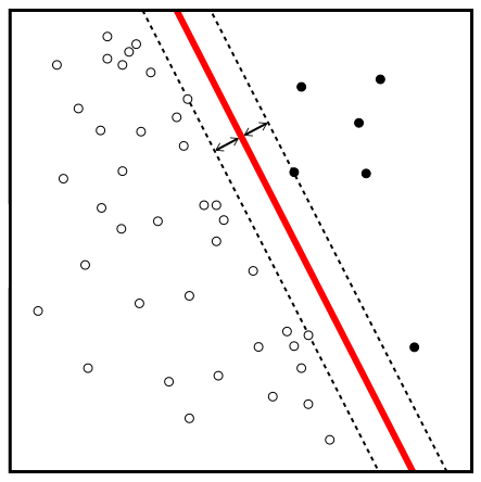
Figure 8.3: Maximal margin hyperplane. Source: https://tinyurl.com/y493pww8
The problem in practice is that a separating hyperplane usually doesn’t exist. Even if a separating hyperplane existed, we may not want to use the maximal margin hyperplane as it would perfectly classify all of the observations and may be too sensitive to individual observations and subsequently overfitting.
Figure 8.4 from James, et al. (2013) clearly illustrates this problem. The left figure shows the maximal margin hyperplane (solid) in a completely separable solution. The figure on the right shows that when a new observation is introduced that the maximal margin hyperplane (solid) shifts rather dramatically relative to its original location (dashed).
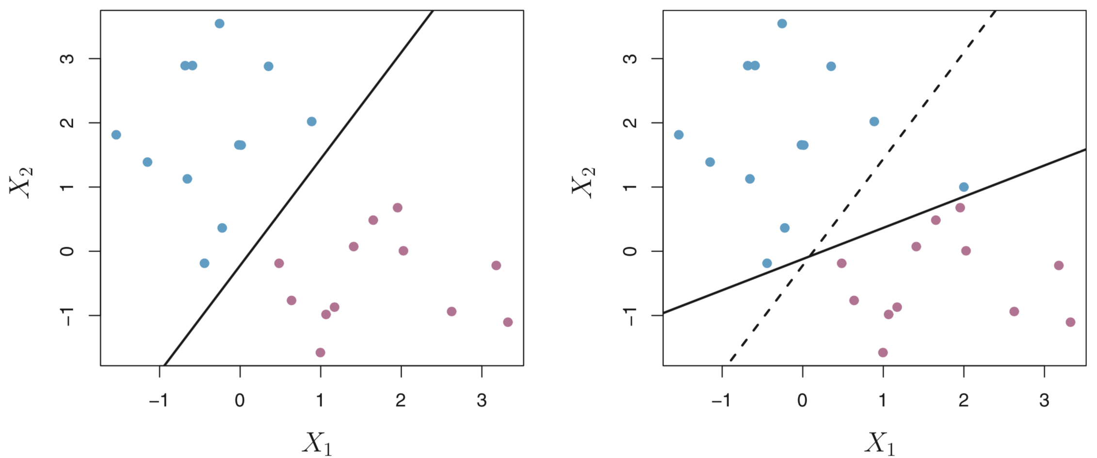
Figure 8.4: The impact of adding one observations to the maximal margin hyperplane from James et al. (2013).
8.1.2 Support Vector Classifier
Our hope for a hyperplane is that it would be relatively insensitive to individual observations, while still classifying training observations well. That is, we would like to have what is termed a soft margin classifier or a support vector classifier. Essentially, we are willing to allow some observations to be on the incorrect side of the margin (classified correctly) or even the incorrect side of the hyperplane (incorrectly classified) if our classifier, overall, performs well.
We do this by introducing a tuning parameter, C, which determines the number and the severity of violations to the margin/hyperplane we are willing to tolerate. As C increases, our tolerance for violations will increase and subsequently our margin will widen. C, thus, represents a bias-variance tradeoff, when C is small bias should be low, but variance will likely be high, whereas when C is large, bias is likely high but our variance is typically small. C will be selected, optimally, through cross-validation (as we’ll see later).
The observations that lie on the margin or violate the margin are the only ones that will affect the hyperplane and the classifier (similar to the maximal margin classifier). These observations are the support vectors and only they will affect the support vector classifier. When C is large, there will be many support vectors, whereas when C is small, the number of support vectors will be less.
Because the support vector classifier depends on only the on the support vectors (which could be very few) this means they are quite robust to the observations that are far from the hyperplane. This makes this technique similar to logistic regression.
8.1.2.1 Example
In our example, we’ll try and classify whether someone scores at or above the mean on the science scale we created earlier. To do support vector classifiers (and SVMs) in R, we’ll use the e1071 package (though the caret package could be used, too).
# check if e1071 is installed
# if not, install it
if (!("e1071" %in% installed.packages()[,"Package"])) {
  install.packages("e1071")
  library("e1071")
} else {
  library("e1071")
}
The svm function in the e1071 package requires that the outcome variable is a factor. So, we’ll do a mean split (at the OECD mean of 493) on the science scale and convert it to a factor.
pisa[, sci_class := as.factor(ifelse(science >= 493, 1, -1))]While, I’m coding this variable as 1 and -1 to be consistent with the notation above, it doesn’t matter to the svm function. The only thing the svm function needs to perform classification and not regression is that the outcome is a factor. If the outcome has just two values, a 1 and -1, but is not a factor, svm will perform regression.
We will use the following variables in our model:
| Label | Description |
|---|---|
| WEALTH | Family wealth (WLE) |
| HEDRES | Home educational resources (WLE) |
| ENVAWARE | Environmental Awareness (WLE) |
| ICTRES | ICT Resources (WLE) |
| EPIST | Epistemological beliefs (WLE) |
| HOMEPOS | Home possessions (WLE) |
| ESCS | Index of economic, social and cultural status (WLE) |
| reading | Reading score |
| math | Math score |
We’ll subset the variables to make it easier and in order for the model fitting to be performed in a reasonable amount of time in R, we’ll just subset the United States and Canada.
pisa_sub <- subset(pisa, CNT %in% c("Canada", "United States"), select = c(sci_class, WEALTH, HEDRES, ENVAWARE, ICTRES, EPIST, HOMEPOS, ESCS, reading, math))To fit a support vector classier, we use the svm function. Before we get started, let’s divide the data set into a training and a testing data set. We will use a 66/33 split, though other splits could be used (e.g., 50/50).
# set a random seed
set.seed(442019)

# svm uses listwise deletion, so we should just drop
# the observations now
pisa_m <- na.omit(pisa_sub)

# select the rows that will go into the training data set.
train <- sample(1:nrow(pisa_m), 2/3 * nrow(pisa_m))

# subset the data based on the rows that were selected to be in training data set.
train_dat <- pisa_m[train, ]
test_dat <- pisa_m[-train, ]
To perform support vector classification, we pass the svm function the kernel = "linear" argument. We also need to specify our tolerance, which is represented by the cost argument. The cost parameter is essentially the inverse of the tolerance parameter, C, described above. When the cost value is low, the tolerance is high (i.e., the margin is wide and there are lots of support vectors) and when the cost value is high, the tolerance is low (i.e., narrower margin). By default cost = 1 and we will tune this parameter via cross-validation momentarily. For now, we’ll just fit the model.
svc_fit <- svm(sci_class ~., data = train_dat, kernel = "linear")We can obtain basic information about our model using the summary function.
summary(svc_fit)##
## Call:
## svm(formula = sci_class ~ ., data = train_dat, kernel = "linear")
##
##
## Parameters:
## SVM-Type: C-classification
## SVM-Kernel: linear
## cost: 1
## gamma: 0.1111111
##
## Number of Support Vectors: 2782
##
## ( 1390 1392 )
##
##
## Number of Classes: 2
##
## Levels:
## -1 1We see there are 2782 support vectors: 1390 in class -1 and 1392 in class 1. We can also plot our model but we need to specific the two features we want to plot (because our model has nine feature). Let’s look at the model with math on the y-axis and reading on the x-axis.
plot(svc_fit, data = train_dat, math ~ reading)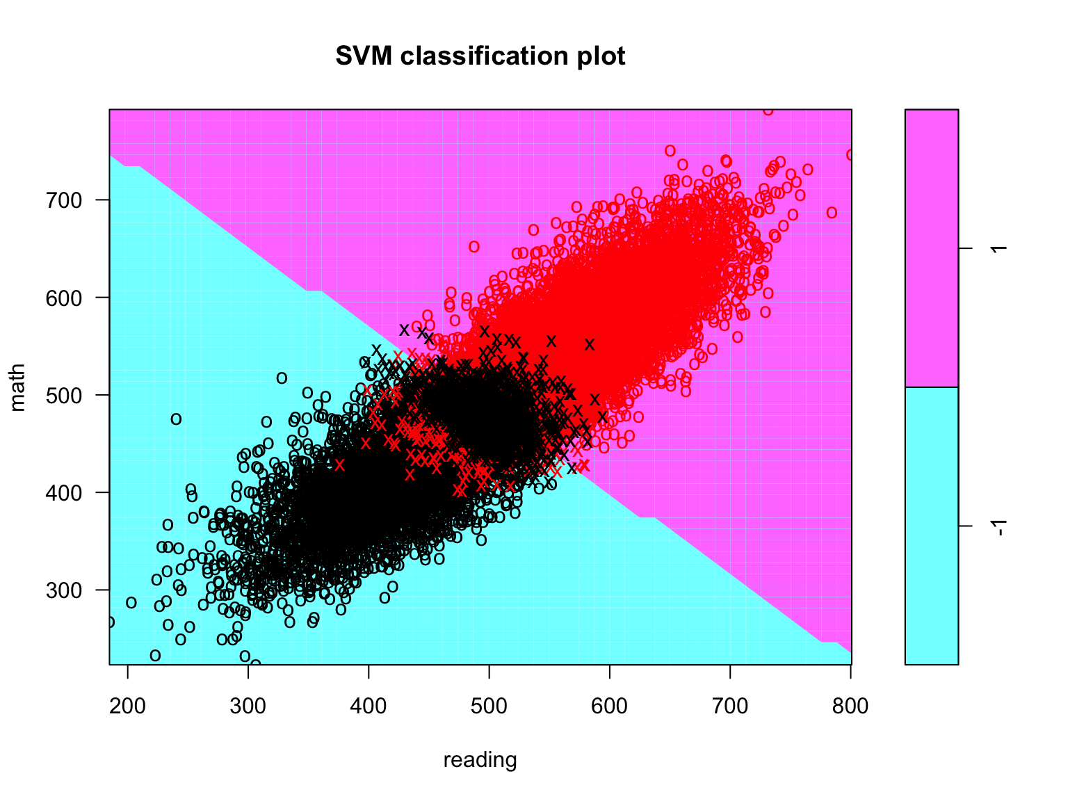
Figure 8.5: Support vector classifier plot for all the training data.
In this figure, the red points correspond to observations that belong to class 1 (below the mean on science), while the black points correspond to observations that belong to class -1 (at/above the mean on science); the Xs are the support vectors, while the Os are the non-support vector observations; the upper triangle (purple) are for class 1, while the lower triangle (blue) is for class -1. While the decision boundary looks jagged, it’s just an artifact of the way it’s drawn with this function. We can see that many observations are misclassified (i.e., some red points are in the lower triangle and some black points are in the upper triangle). However, there are a lot of observations shown in this figure and it is difficult to discern the nature of the misclassification.
As was discussed in the section on data visualization, with this many points on a figure it is difficult to evaluate patterns, not to mention that the figure is extremely slow to render. Therefore, let’s take a random sample of 1,000 observations to get a better sense of our classifier. This is shown in Figure 8.6.
set.seed(1)
ran_obs <- sample(1:nrow(train_dat), 1000)
plot(svc_fit, data = train_dat[ran_obs, ], math ~ reading)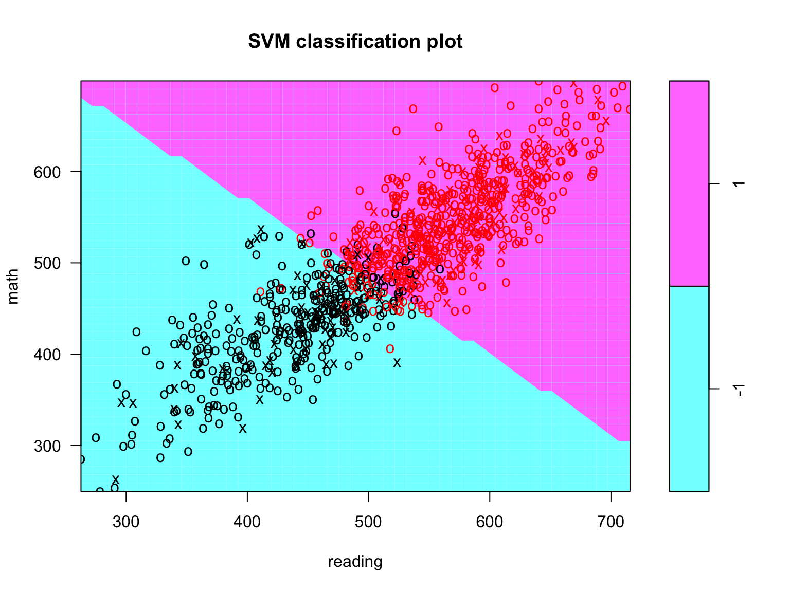
Figure 8.6: Support vector classifier plot for all a random subsample (n = 1000) of training observations.
Notice that few points are crossing the hyperplane (i.e., are misclassified). This looks like the classier is doing pretty good.
Initially when we fit the support vector classifier we used the default cost parameter, but we really should select this parameter through tuning via cross-validation as we might be able to do an even better job at classifying. The e1071 package includes a tune function which makes this easy and automatic. It performs the tuning via 10-folds cross-validation by default, which is probably a fine tradeoff (see James, et al. 2013 for a comparison of k-folds vs. leave one out cross-validation). We need to provide the tune function with a range of cost values (which again corresponds to our tolerance to violate the margin and hyperplane).
tune_svc <- tune(svm, sci_class ~., data = train_dat,
                 kernel="linear",
                 ranges = list(cost = c(.01, .1, 1, 5, 10)))
On my Macbook Pro (2.6 GHz Intel Core i7 and 16 GB RAM) it takes approximately 2 minutes run this. Without doing this subsetting, it will take quite a bit longer to do.
We can view the cross-validation errors by using the summary function on this object.
summary(tune_svc)##
## Parameter tuning of 'svm':
##
## - sampling method: 10-fold cross validation
##
## - best parameters:
## cost
## 1
##
## - best performance: 0.07316727
##
## - Detailed performance results:
## cost error dispersion
## 1 0.01 0.07342096 0.005135708
## 2 0.10 0.07354766 0.004985649
## 3 1.00 0.07316727 0.004952085
## 4 5.00 0.07329406 0.004879146
## 5 10.00 0.07335747 0.004887063And then select the best model and view it.
best_svc <- tune_svc$best.model
summary(best_svc)
##
## Call:
## best.tune(method = svm, train.x = sci_class ~ ., data = train_dat,
## ranges = list(cost = c(0.01, 0.1, 1, 5, 10)), kernel = "linear")
##
##
## Parameters:
## SVM-Type: C-classification
## SVM-Kernel: linear
## cost: 1
## gamma: 0.1111111
##
## Number of Support Vectors: 2782
##
## ( 1390 1392 )
##
##
## Number of Classes: 2
##
## Levels:
## -1 1Next, we write a function to evaluate our classifier that has one argument that takes a confusion matrix.
#' Evaluate classifier
#'
#' Evaluates a classifier (e.g. SVM, logistic regression)
#' @param tab a confusion matrix
eval_classifier <- function(tab, print = F){
  n <- sum(tab)
  TP <- tab[2,2]
  FN <- tab[2,1]
  FP <- tab[1,2]
  TN <- tab[1,1]
  classify.rate <- (TP + TN) / n
  TP.rate <- TP / (TP + FN)
  TN.rate <- TN / (TN + FP)
  object <- data.frame(accuracy = classify.rate,
                       sensitivity = TP.rate,
                       specificity = TN.rate)
  object
}
The confusion matrix is just a list of all possible outcomes (true positives, true negatives, false positives, and false negatives). A confusion matrix for our best_svc can be created by:
# to create a confusion matrix this order is important!
# observed values first and predict values second!
svc_cm_train <- table(train_dat$sci_class,
                      predict(best_svc))
svc_cm_train
##
## -1 1
## -1 5563 606
## 1 550 9053The top-left are the true negatives, the bottom-left are the false negatives, the top-right are the false positives, and the bottom-right are the true positives. We can request the accuracy (the % of observations that were correctly classified), the sensitivity (the % of observations that were in class 1 that were correctly identified), and specificity (the % of observations that were in class -1 that were correctly identified) using the eval_classifier function.
eval_classifier(svc_cm_train)## accuracy sensitivity specificity
## 1 0.9267056 0.9427262 0.9017669Performance is pretty good overall. We see that class -1 (specificity) isn’t classified as well as class 1 (sensitivity). These statistics are likely overly optimistic as we are evaluating our model using the training data (the same data that we used to build our model). How well does the model perform on the testing data?
svc_cm_test <- table(test_dat$sci_class,
                     predict(best_svc, newdata = test_dat))
svc_cm_test
##
## -1 1
## -1 2780 281
## 1 278 4547eval_classifier(svc_cm_test)## accuracy sensitivity specificity
## 1 0.9291149 0.9423834 0.9081999Still impressively high! This is a very good classifier indeed. This is likely because math and reading are so highly correlated with science scores.
We can extract the coefficients from our model that make up our decision boundary.
beta0 <- best_svc$rho
beta <-  drop(t(best_svc$coefs) %*% as.matrix(train_dat[best_svc$index, -1]))
beta0
## [1] -1.220883beta## WEALTH HEDRES ENVAWARE ICTRES EPIST
## 0.04398688 -0.24398165 0.36167882 -0.09803825 0.04652237
## HOMEPOS ESCS reading math
## 0.22005477 -0.15065808 188.02960807 196.93421586With more complicated SVMs with non-linear kernels, coefficients don’t make any sense and generally are of little interest with applying these models.
8.1.2.2 Comparison to logistic regression
Support vector classifiers are quite similar to logistic regression. This has to do with them having similar loss functions (the functions used to estimate the parameters). In situations where the classes are well separated, SVM (more generally), tend to do better than logistic regression and when they are not well separated, logistic regression tends to do better (James, et al., 2013).
Let’s compare logistic regression to the support vector classier. We’ll begin by fitting the model
lr_fit <- glm(sci_class ~. , data = train_dat, family = "binomial")and then viewing the coefficients.
coef(lr_fit)## (Intercept) WEALTH HEDRES ENVAWARE ICTRES
## -41.82682653 0.11666541 -0.26667828 0.30159987 -0.13594566
## EPIST HOMEPOS ESCS reading math
## 0.05053261 0.20699211 -0.24568642 0.03917470 0.04651408How does it do relative to our best support vector classifier on the training and the testing data sets? For the training data set
lr_cm_train <- table(train_dat$sci_class,
                     round(predict(lr_fit, type = "response")))
lr_cm_train
##
## 0 1
## -1 5567 602
## 1 541 9062eval_classifier(lr_cm_train)## accuracy sensitivity specificity
## 1 0.9275298 0.9436634 0.9024153and then for the testing data set.
lr_cm_test <- table(test_dat$sci_class,
                     round(predict(lr_fit, newdata = test_dat, type = "response")))
lr_cm_test
##
## 0 1
## -1 2780 281
## 1 275 4550eval_classifier(lr_cm_test)## accuracy sensitivity specificity
## 1 0.9294953 0.9430052 0.9081999Equivalent out to the hundredths place. Either model would be fine here.
8.1.2.3 Using Apache Spark for machine learning
Apache Spark is also capable of running support vector classifiers. It does this using the ml_linear_svc function. The amazing thing about this is that you can use it to run the entire data set (i.e., there is no need to subset out a portion of the countries). If we tried to do this with the e1071 package it would be very impractical and take forever, but with Apache Spark it is feasible and reasonably quick (just a few minutes).
We’ll again use the sparklyr package to interface with Spark and use the dplyr package to simplify interacting with Spark.
library(sparklyr)
library(dplyr)
We first need to establish a connection with Spark and then copy a subsetted PISA data set to Spark.
sc <- spark_connect(master = "local")
spark_sub <- subset(pisa,
                    select = c(sci_class, WEALTH, HEDRES, ENVAWARE, ICTRES,
                               EPIST, HOMEPOS, ESCS, reading, math))
spark_sub <- na.omit(spark_sub) # can't handle missing data
pisa_tbl <- copy_to(sc, spark_sub, overwrite = TRUE)
Now, we’ll let Spark partition the data into a training and a test data set.
partition <- pisa_tbl %>%
  sdf_partition(training = 2/3, test = 1/3, seed = 442019)
pisa_training <- partition$training
pisa_test <- partition$test
We are ready to run the classifier in Spark. Unlike the svm function, the tolerance parameter is called reg_param. This parameter should be optimally selected like it was for svm. By default the tolerance is 1e-06.
svc_spark <- pisa_training %>%
  ml_linear_svc(sci_class ~ .)
We then use the ml_predict function to predict the classes.
svc_pred <- ml_predict(svc_spark, pisa_training) %>%
  select(sci_class, predicted_label) %>%
  collect()
Then print the confusion matrix and the criteria that we’ve been using to evaluate our models.
table(svc_pred)## predicted_label
## sci_class -1 1
## -1 145111 12353
## 1 10753 121967eval_classifier(table(svc_pred))## accuracy sensitivity specificity
## 1 0.9204 0.919 0.9216Again, this is really good. How does it look on the testing data?
svc_pred_test <- ml_predict(svc_spark, pisa_test) %>%
  select(sci_class, predicted_label) %>%
collect()table(svc_pred_test)## predicted_label
## sci_class -1 1
## -1 72577 6199
## 1 5438 60953eval_classifier(table(svc_pred_test))## accuracy sensitivity specificity
## 1 0.9198 0.9181 0.9213Pretty impressive. We can also Apache Spark to fit logistic regression using the ml_logistic_regression function.
spark_lr <- pisa_training %>%
  ml_logistic_regression(sci_class ~ .)
And view the performance on the training and test data sets.
## Training data
svc_pred_lr <- ml_predict(spark_lr, pisa_training) %>%
  select(sci_class, predicted_label) %>%
  collect()
table(svc_pred_lr)
## predicted_label
## sci_class -1 1
## -1 146217 11247
## 1 11133 121587eval_classifier(table(svc_pred_lr))## accuracy sensitivity specificity
## 1 0.9229 0.9161 0.9286## Test data
svc_pred_test_lr <- ml_predict(spark_lr, pisa_test) %>%
select(sci_class, predicted_label) %>%
collect()
table(svc_pred_test_lr)## predicted_label
## sci_class -1 1
## -1 73098 5678
## 1 5646 60745eval_classifier(table(svc_pred_test_lr))## accuracy sensitivity specificity
## 1 0.922 0.915 0.9279We could also use the logistic regression in R as it’s pretty quick even with this large of a data set (in fact, it’s slightly quicker).
Finally, it is quite common to evaluate these models using AUC. We can let Apache Spark do this for the test data sets.
# extract predictions
pred_svc <- ml_predict(svc_spark, pisa_test)
pred_lr <- ml_predict(spark_lr, pisa_test)

ml_binary_classification_evaluator(pred_svc)
## [1] 0.9795ml_binary_classification_evaluator(pred_lr)## [1] 0.9805We want these values as close to 1 as a possible. These values are all quite large and corroborate that these are both good classifiers.
8.1.3 Support Vector Machine
SVM is an extension of support vector classifiers using kernels that allow for a non-linear boundary between the classes. Without getting into the weeds, to solve a support vector classifier problem all you need to know is the inner products of the observations. Assuming that \(x_i\) and \(x_i'\) are two observations and \(p\) is the number of predictors (features), their inner product is defined as:
\[ \langle x_i, x_i'\rangle = \begin{bmatrix} x_{i1} x_{i2} \dots x_{ip} \end{bmatrix} \begin{bmatrix} x_{i1}' \\ x_{i2}' \\ \vdots \\ x_{ip}' \end{bmatrix} = x_{i1}x_{i1}' + x_{i2}x_{i2}' + \dots x_{ip}x_{ip}' \]
More succinctly, \(\langle x_i, x_i'\rangle = \sum_{i = 1}^p x_{ij}x_{ij}'\). We can replace the inner product with a more general form, \(K(x_i, x_i')\), where \(K\) is a kernel (a function that quantifies the similarity of two observations). When,
\[ K(x_i, x_i') = \sum_{i = 1}^p x_{ij}x_{ij} \]
We have the linear kernel and this is the support vector classifier. However, we can use a more flexible kernel. Such as:
\[ K(x_i, x_i') = (1 + \sum_{i = 1}^p x_{ij}x_{ij})^d \]
which is known as a polynomial kernel of degree \(d\) and when \(d > 1\) we have much more flexible decision boundary than we do for support vector classifiers (when \(d = 1\) we are back to the support vector classifier).
Another very common kernel is the radial kernel, which is given by:
\[ K(x_i, x_i') = \exp\left(-\gamma \sum_{i = 1}^p (x_{ij} - x_{ij})^2\right) \]
where \(\gamma\) is a positive constant. Note, both \(d\) and \(\gamma\) are selected via tuning and cross-validation.
Both of these kernels are worth considering when the decision boundary is non-linear. Figure 8.7 from James, et al. (2013) gives an example of a non-linear boundary. We see that the classes are not linearly separated and if we tried to use a linear decision boundary, we would end up with a very poor classifier. Therefore, we need to use a more flexible kernel. In both cases, we should expect that an SVM would greatly outperform both a support vector classifier and logistic regression.
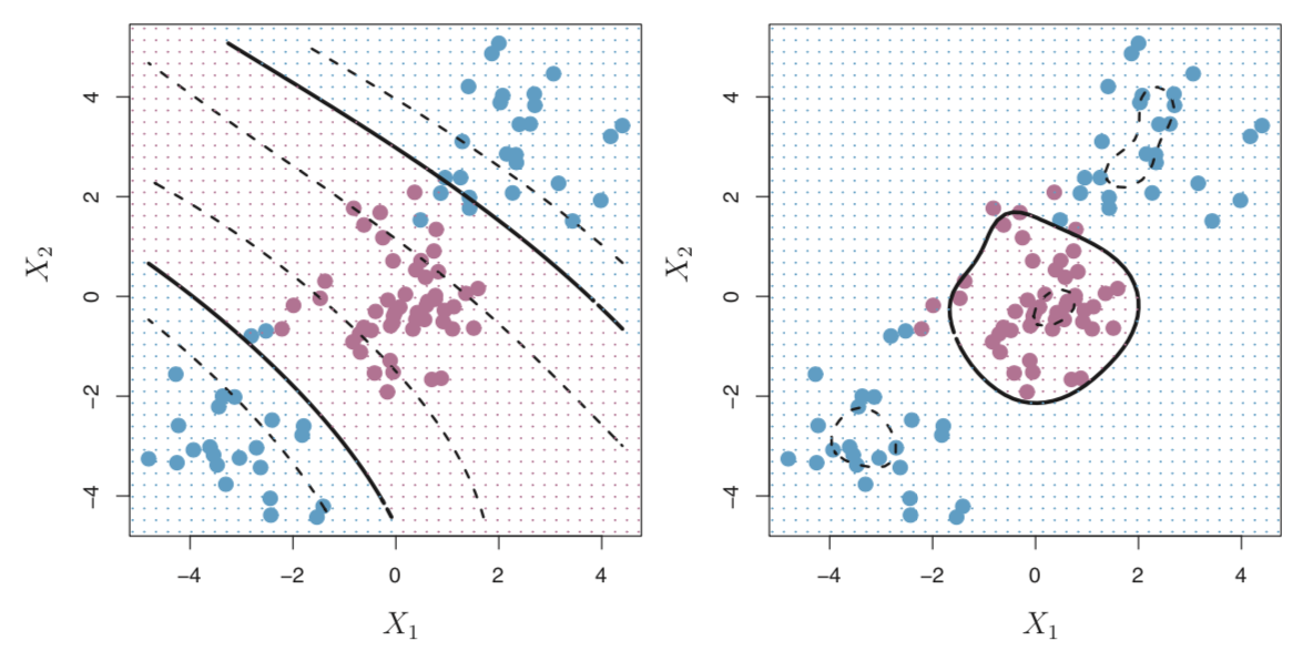
Figure 8.7: Non-linear decision boundary with a polynomial kernel (left) and radial kernel (right) from James et al., 2013.
8.1.3.1 Examples
We will continue trying to build the best classifier of whether someone scored in the upper or lower half on the science scale and again use the svm function in the e1071 package. For brevity, we’ll consider only the radial kernel. By default gamma is set to 1. We’ll explicitly set it to 1 below and cost to 1.
svm_fit <- svm(sci_class ~., data = train_dat,
               cost = 1,
               gamma = 1,
               kernel = "radial")
Again, we can request some basic information about our model.
summary(svm_fit)##
## Call:
## svm(formula = sci_class ~ ., data = train_dat, cost = 1, gamma = 1,
## kernel = "radial")
##
##
## Parameters:
## SVM-Type: C-classification
## SVM-Kernel: radial
## cost: 1
## gamma: 1
##
## Number of Support Vectors: 6988
##
## ( 3676 3312 )
##
##
## Number of Classes: 2
##
## Levels:
## -1 1This time we see we have 6988 support vectors, 3676 in class -1 and 3312 in class 1. Quite a bit more support vectors than the support vector classifier. Lets visually inspect this model by plotting it against the math and reading features on the same subset of test takers (Figure 8.8.
plot(svm_fit, data = train_dat[ran_obs, ], math ~ reading)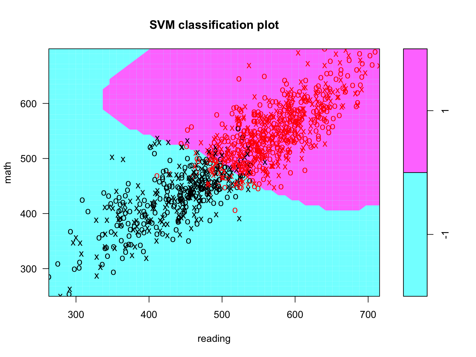
Figure 8.8: Support vector classifier plot for all a random subsample (n = 1000) of training observations.
We see that the decision boundary is now clearly no longer linear and we again see decent classification. Before we investigate the fit of the model, we should tune it.
tune_svm <- tune(svm, sci_class ~., data = train_dat,
                 kernel = "radial",
                 ranges = list(cost = c(.01, .1, 1, 5, 10),
                               gamma = c(0.5, 1, 2, 3, 4)))
We can see which model was selected
summary(tune_svm)##
## Parameter tuning of 'svm':
##
## - sampling method: 10-fold cross validation
##
## - best parameters:
## cost gamma
## 0.1 0.5
##
## - best performance: 0.07583144
##
## - Detailed performance results:
## cost gamma error dispersion
## 1 0.01 0.5 0.17670590 0.010347886
## 2 0.10 0.5 0.07583144 0.008233504
## 3 1.00 0.5 0.07754307 0.009223528
## 4 5.00 0.5 0.08375680 0.008098257
## 5 10.00 0.5 0.08718054 0.008157393
## 6 0.01 1.0 0.36425229 0.011955406
## 7 0.10 1.0 0.13162657 0.007210614
## 8 1.00 1.0 0.08242504 0.008590571
## 9 5.00 1.0 0.09402859 0.009848512
## 10 10.00 1.0 0.10074908 0.007984562
## 11 0.01 2.0 0.39113500 0.011126599
## 12 0.10 2.0 0.31409966 0.010609909
## 13 1.00 2.0 0.11469785 0.006880824
## 14 5.00 2.0 0.12363760 0.006591525
## 15 10.00 2.0 0.12465198 0.006523243
## 16 0.01 3.0 0.39113500 0.011126599
## 17 0.10 3.0 0.38257549 0.012981991
## 18 1.00 3.0 0.17562831 0.007488136
## 19 5.00 3.0 0.17277475 0.006502038
## 20 10.00 3.0 0.17309173 0.006145790
## 21 0.01 4.0 0.39113500 0.011126599
## 22 0.10 4.0 0.39107163 0.011072976
## 23 1.00 4.0 0.23960159 0.011545434
## 24 5.00 4.0 0.22641364 0.008709051
## 25 10.00 4.0 0.22641360 0.008779341And then select the best model and view it.
best_svm <- tune_svm$best.model
summary(best_svm)
##
## Call:
## best.tune(method = svm, train.x = sci_class ~ ., data = train_dat,
## ranges = list(cost = c(0.01, 0.1, 1, 5, 10), gamma = c(0.5,
## 1, 2, 3, 4)), kernel = "radial")
##
##
## Parameters:
## SVM-Type: C-classification
## SVM-Kernel: radial
## cost: 0.1
## gamma: 0.5
##
## Number of Support Vectors: 6138
##
## ( 3095 3043 )
##
##
## Number of Classes: 2
##
## Levels:
## -1 1Finally, we see how well this predicts on both the training observations
svm_cm_train <- table(train_dat$sci_class,
                     predict(best_svm))
svm_cm_train
##
## -1 1
## -1 5620 549
## 1 519 9084eval_classifier(svm_cm_train)## accuracy sensitivity specificity
## 1 0.9322851 0.9459544 0.9110066and finally the testing observations.
svm_cm_test <- table(test_dat$sci_class,
                     predict(best_svm, newdata = test_dat))
svm_cm_test
##
## -1 1
## -1 2781 280
## 1 291 4534eval_classifier(svm_cm_test)## accuracy sensitivity specificity
## 1 0.9275932 0.9396891 0.9085266Performance is very comparable to the support vector classifier and logistic regression implying there isn’t much gain from the use of non-linear decision boundary.
8.1.4 Lab
For the lab, we’ll try to build the best classifier for the “Do you expect your child will go into a
Split the data into a training and a testing data set. Rather than using a 66/33 split, try a 50/50 or a 75/25 split.
Fit a decision tree or random forest
- Prune your model and plot your model (if using decision trees)
- Determine the ideal number of trees (if using random forests)
- Fit a support vector machine
- Consider different kernels (e.g., linear and radial)
- Visually inspect your model by plotting it against a few features. Create a few different plots.
- Tune the parameters.
- How many support vectors do you have?
- Did you notice much difference in the error rates?
- Does your model have a high tolerance?
- (OPTIONAL): When fitting the support vector classifier, you could try and fit it using Apache Spark
- If you do this, use the
ml_binary_classification_evaluatorfunction to calculate AUC.
- If you do this, use the
- Run a logistic regression
- Examine the coefficients table
- Evaluate the fit of your models using the
eval_classifierfunction on the testing data.
- Which model(s) fits the best? Can you improve it?
- Record your accuracy, sensitivity, and specificity for all the models (decision tree or random forest and SVM) to share.
The following table contains the list of variables you could consider (this were introduced earlier):
| Label | Description |
|---|---|
| DISCLISCI | Disciplinary climate in science classes (WLE) |
| TEACHSUP | Teacher support in a science classes of students choice (WLE) |
| IBTEACH | Inquiry-based science teaching an learning practices (WLE) |
| TDTEACH | Teacher-directed science instruction (WLE) |
| ENVAWARE | Environmental Awareness (WLE) |
| JOYSCIE | Enjoyment of science (WLE) |
| INTBRSCI | Interest in broad science topics (WLE) |
| INSTSCIE | Instrumental motivation (WLE) |
| SCIEEFF | Science self-efficacy (WLE) |
| EPIST | Epistemological beliefs (WLE) |
| SCIEACT | Index science activities (WLE) |
| BSMJ | Student’s expected occupational status (SEI) |
| MISCED | Mother’s Education (ISCED) |
| FISCED | Father’s Education (ISCED) |
| OUTHOURS | Out-of-School Study Time per week (Sum) |
| SMINS | Learning time (minutes per week) - |
| TMINS | Learning time (minutes per week) - in total |
| BELONG | Subjective well-being: Sense of Belonging to School (WLE) |
| ANXTEST | Personality: Test Anxiety (WLE) |
| MOTIVAT | Student Attitudes, Preferences and Self-related beliefs: Achieving motivation (WLE) |
| COOPERATE | Collaboration and teamwork dispositions: Enjoy cooperation (WLE) |
| PERFEED | Perceived Feedback (WLE) |
| unfairteacher | Teacher Fairness (Sum) |
| HEDRES | Home educational resources (WLE) |
| HOMEPOS | Home possessions (WLE) |
| ICTRES | ICT Resources (WLE) |
| WEALTH | Family wealth (WLE) |
| ESCS | Index of economic, social and cultural status (WLE) |
| math | Students’ math scores |
| reading | Students’ reading scores |