3 Data Wrangling
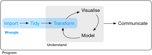
Nearly all datasets require some initial procedures (e.g., cleaning, reformatting, reshaping) to be applied before we start running any statistical analysis or creating visualizations. These procedures are often referred to as data wrangling. Here is a nice summary of the data wrangling process:

Data wrangling process [Source: Grolemund and Wickham (2018)]
In this section, we will follow the steps of data wrangling as shown above.
3.1 Creating Datasets in R
There are multiple ways of creating datasets in R. We can create individual variables and combine them using the cbind (column bind) command:
age <- c(21, 24, 32, 45, 52)
salary <- c(4500, 3500, 4100, 4700, 6000)
mydata <- cbind(age, salary)
mydata
age salary
[1,] 21 4500
[2,] 24 3500
[3,] 32 4100
[4,] 45 4700
[5,] 52 6000We can also create individual rows and combine them using the rbind (row bind) command (though this is not practical if there are many rows):
person1 <- c(21, 4500)
person2 <- c(24, 3500)
person3 <- c(32, 4100)
person4 <- c(45, 4700)
person5 <- c(52, 6000)

mydata <- rbind(person1, person2, person3, person4, person5)
mydata
[,1] [,2]
person1 21 4500
person2 24 3500
person3 32 4100
person4 45 4700
person5 52 6000A better way to create datasets in R is to define variables within a data frame using the data.frame command.
mydata <- data.frame(age = c(21, 24, 32, 45, 52),
                     salary = c(4500, 3500, 4100, 4700, 6000))
mydata
age salary
1 21 4500
2 24 3500
3 32 4100
4 45 4700
5 52 6000Data frames in R are very convenient because many mathematical operations can be directly applied to a data frame or some columns (or rows) of a data frame. Once a data frame is defined in R, we can see its content using the View command (which open the data window) or the head command (which prints the first six rows of the data):
# To print the first six rows of a data frame
head(mydata)

# To see the entire data in the view window
View(mydata)
3.2 Importing Data into R
We often save our data sets in convenient data formats, such as Excel, SPSS, or text files (.txt, .csv, .dat, etc.). R is capable of importing (i.e., reading) various data formats.
There are two ways to import a data set into R:
- By using the “Import Dataset” menu option in RStudio
- By using a particular R command
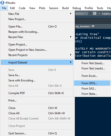
3.2.1 Method 1: Using RStudio

Importing a dataset using the RStudio menu
3.2.1.1 Importing Excel Files
- Browse for the file that you want to import
- Give a name for the data set
- Choose the sheet to be imported
- “First Row as Names” if the variable names are in the first row of the file.

Importing Excel files
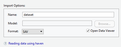
3.2.1.2 Importing SPSS Files
- Browse the file that you want to import
- Give a name for the data set
- Choose the SPSS data format (SAV)

Importing SPSS files
3.2.2 Method 2: Using R Commands
R has some built-in functions, such as read.csv and read.table. Also, there are R packages for importing specific data formats. For example, foreign for SPSS files and xlsx for Excel files. Here are some examples:
Excel Files:
# Install and activate the package first
install.packages("xlsx")
library("xlsx")

# Use read.xlsx to import an Excel file
my_excel_file <- read.xlsx("path to the file/filename.xlsx", sheetName = "sheetname")
SPSS Files:
# Install and activate the package first
install.packages("foreign")
library("foreign")

# Use read.spss to import an SPSS file
my_spss_file <- read.spss("path to the file/filename.sav", to.data.frame = TRUE)
Text Files:
# No need to install any packages
# R has many built-in functions already

# A comma-separated-values file with a .csv extension
my_csv_file <- read.csv("path to the file/filename.csv", header = TRUE)

# A tab delimited text file with .txt extension
my_txt_file <- read.table("path to the file/filename.txt", header = TRUE, sep = "\t")
Here we should note that:
header = TRUEif the variable names are in the first row; otherwise, useheader = FALSEsep="\t"for tab-separated files;sep=","for comma-separated files
3.2.3 Exercise 3
Now we will import the medical dataset into R. The dataset comes from a clinical study. Patients with no primary care physician were randomized to receive a multidisciplinary assessment and a brief motivational intervention, with the goal of linking them to primary medical care. You can find the details in “Codebook for the medical Dataset” in your folder. Our dataset is in a .csv format (medical.csv).
- Import the file
medical.csvby using theread.csvcommand and save it asmedicalusing the following code (assuming that the file is in your working directory):
medical <- read.csv("medical.csv", header = TRUE)- Once the data file is successfully imported, run the following to see the first six rows of the data:
head(medical)You should be able to see the output below:
  id age    sex  race homeless substance avg_drinks max_drinks suicidal treat
1  1  37   male black   housed   cocaine         13         26      yes   yes
2  2  37   male white homeless   alcohol         56         62      yes   yes
3  3  26   male black   housed    heroin          0          0       no    no
4  4  39 female white   housed    heroin          5          5       no    no
5  5  32   male black homeless   cocaine         10         13       no    no
6  6  47 female black   housed   cocaine          4          4       no   yes
  physical1 mental1 depression1 physical2 mental2 depression2
1     58.41  25.112          49     54.23   52.23           7
2     36.04  26.670          30     59.56   41.73          11
3     74.81   6.763          39     58.46   56.77          14
4     61.93  43.968          15     46.61   14.66          44
5     37.35  21.676          39     31.42   40.67          26
6     46.48  55.509           6     43.20   50.06          23
3.3 Understanding the Data
After we import a dataset into R, we can quickly check a few things to understand our dataset better:
- To see the number of rows in the data:
nrow(medical)[1] 246- To see the number of columns in the data:
ncol(medical)[1] 16- To see its dimensions all together:
dim(medical)[1] 246 16- To see all of the variable names in the data:
names(medical) [1] "id" "age" "sex" "race" "homeless"
[6] "substance" "avg_drinks" "max_drinks" "suicidal" "treat"
[11] "physical1" "mental1" "depression1" "physical2" "mental2"
[16] "depression2"- To see the structure of the entire dataset:
str(medical)'data.frame': 246 obs. of 16 variables:
$ id : int 1 2 3 4 5 6 8 9 10 12 ...
$ age : int 37 37 26 39 32 47 28 50 39 58 ...
$ sex : chr "male" "male" "male" "female" ...
$ race : chr "black" "white" "black" "white" ...
$ homeless : chr "housed" "homeless" "housed" "housed" ...
$ substance : chr "cocaine" "alcohol" "heroin" "heroin" ...
$ avg_drinks : int 13 56 0 5 10 4 12 71 20 13 ...
$ max_drinks : int 26 62 0 5 13 4 24 129 27 13 ...
$ suicidal : chr "yes" "yes" "no" "no" ...
$ treat : chr "yes" "yes" "no" "no" ...
$ physical1 : num 58.4 36 74.8 61.9 37.3 ...
$ mental1 : num 25.11 26.67 6.76 43.97 21.68 ...
$ depression1: int 49 30 39 15 39 6 32 50 46 49 ...
$ physical2 : num 54.2 59.6 58.5 46.6 31.4 ...
$ mental2 : num 52.2 41.7 56.8 14.7 40.7 ...
$ depression2: int 7 11 14 44 26 23 18 33 37 8 ...3.4 Indexing
In R, each row and column is indexed by the position they appear in the data. R uses square brackets for indexing. Within the square brackets, the first number shows the row number(s) and the second number shows the column(s). To call a particular column (i.e., variables) or a particular row (i.e., persons), we can use the following structure: data[row, col]
For example, if we want to see the second variable for the fifth person in the medical dataset:
medical[5, 2][1] 32Or, if we want to see the first three variables for the first five persons:
medical[1:5, 1:3] id age sex
1 1 37 male
2 2 37 male
3 3 26 male
4 4 39 female
5 5 32 maleInstead of medical[1:5, 1:3], we could also do:
medical[c(1, 2, 3, 4, 5), c(1, 2, 3)] id age sex
1 1 37 male
2 2 37 male
3 3 26 male
4 4 39 female
5 5 32 maleor
medical[c(1, 2, 3, 4, 5), c("id", "age", "sex")] id age sex
1 1 37 male
2 2 37 male
3 3 26 male
4 4 39 female
5 5 32 maleA common way of indexing variables (i.e., columns) in R is to use the dollar sign with a variable name from a data frame. For example, we can select the age variable as follows:
medical$ageThis would print all the values for age in the medical dataset. We can also preview a particular variable using the head function.
head(medical$age)[1] 37 37 26 39 32 47Using a particular variable, we can also see the values for some rows in the data. For example, let’s print the age variable for the 10th to 15th rows in the medical dataset.
medical$age[10:15]

# or

medical$age[c(10, 11, 12, 13, 14, 15)]
Note that now the brackets don’t need a comma inside as we had before. This is because we have already selected a variable (age) and so R knows that we now refer to rows when we type any values inside the brackets.
3.5 Subsetting
Now assume that we want to create a new dataset with only females from the medical dataset. Although we can subset the data in many ways, the following two are the easiest:
- Using the
subsetfunction in base R:
medical_female <- subset(medical, sex == "female")
head(medical_female)
id age sex race homeless substance avg_drinks max_drinks suicidal
4 4 39 female white housed heroin 5 5 no
6 6 47 female black housed cocaine 4 4 no
8 9 50 female white homeless alcohol 71 129 no
10 12 58 female black housed alcohol 13 13 no
14 17 28 female hispanic homeless heroin 0 0 yes
17 20 27 female white housed heroin 9 24 yes
treat physical1 mental1 depression1 physical2 mental2 depression2
4 no 61.93 43.97 15 46.61 14.66 44
6 yes 46.48 55.51 6 43.20 50.06 23
8 no 38.27 22.03 50 45.56 28.88 33
10 no 41.93 13.38 49 52.96 51.45 8
14 yes 44.78 29.80 35 52.69 46.59 19
17 yes 37.45 15.46 52 61.40 41.53 15Here we use a single selection criterion as sex == "female". We can also subset the data based on multiple criteria and select only some variables from our original data. Let’s assume that we want to select participants who are female and 40 years old or older. Also, we only want to keep the following variables in the dataset: id, age, sex, substance. Using the subset function, we can do this selection as follows:
medical_f40 <- subset(medical, sex == "female" & age >= 40,
                      select = c("id", "age", "sex", "substance"))

head(medical_f40)
id age sex substance
6 6 47 female cocaine
8 9 50 female alcohol
10 12 58 female alcohol
21 27 48 female cocaine
51 65 41 female alcohol
56 71 40 female alcohol- Using the
filterfunction from thedplyrpackage (an amazing package for data wrangling):
# Install and activate the package first
install.packages("dplyr")
library("dplyr")

medical_female <- filter(medical, sex == "female")
head(medical_female)
id age sex race homeless substance avg_drinks max_drinks suicidal
1 4 39 female white housed heroin 5 5 no
2 6 47 female black housed cocaine 4 4 no
3 9 50 female white homeless alcohol 71 129 no
4 12 58 female black housed alcohol 13 13 no
5 17 28 female hispanic homeless heroin 0 0 yes
6 20 27 female white housed heroin 9 24 yes
treat physical1 mental1 depression1 physical2 mental2 depression2
1 no 61.93 43.97 15 46.61 14.66 44
2 yes 46.48 55.51 6 43.20 50.06 23
3 no 38.27 22.03 50 45.56 28.88 33
4 no 41.93 13.38 49 52.96 51.45 8
5 yes 44.78 29.80 35 52.69 46.59 19
6 yes 37.45 15.46 52 61.40 41.53 15Using the filter and select functions from the dplyr package, we can also subset the dataset based on multiple criteria and select some variables from the dataset:
# Filter the data first
medical_f40 <- filter(medical, sex == "female", age >= 40)

# Select the variables to be keep
medical_f40 <- select(medical_f40, id, age, sex, substance)

# Preview the data
head(medical_f40)
There is also a more practical way to accomplish the same task. Here I will demonstrate %>%, which is called the pipe operator. This operator forwards the result of a function to the next function. This way we can simplify the code without creating many intermediate datasets (see https://uc-r.github.io/pipe for more details on the pipe).
medical_f40 <- medical %>% # Send the medical data to filter
  filter(sex == "female", age >= 40) %>% # Filter the data and send it to select
  select(id, age, sex, substance) # Finally select the data

# Preview the data
head(medical_f40)
id age sex substance
1 6 47 female cocaine
2 9 50 female alcohol
3 12 58 female alcohol
4 27 48 female cocaine
5 65 41 female alcohol
6 71 40 female alcoholHere are most common operators for subsetting:
<Less than>Greater than==Equal to<=Less than or equal to>=Greater than or equal to!=Not equal to%in%Group membership&And|Oris.naIs missing (NA).!is.naIs not missing (NA)
3.6 Other Data Manipulation Tools
Here I will mention the other key functions from the dplyr package. These functions solve the vast majority of data manipulation challenges:
arrange: Reorder data based on values of variablesmutate: Create new variablessummarise: Summarize data by functions of choice
Arrange:
# Reorder the data by age
medical_f40 <- arrange(medical_f40, age)

# Let's see if the ordering worked
head(medical_f40)
id age sex substance
1 71 40 female alcohol
2 65 41 female alcohol
3 75 41 female heroin
4 121 42 female cocaine
5 465 42 female alcohol
6 364 43 female heroin# Reorder the data by age in descending order
medical_f40 <- arrange(medical_f40, desc(age))
# Let's see if the ordering worked
head(medical_f40) id age sex substance
1 12 58 female alcohol
2 181 57 female alcohol
3 264 55 female heroin
4 9 50 female alcohol
5 134 50 female alcohol
6 27 48 female cocaineMutate:
# Create a new variable based on age
medical_f40 <- medical_f40 %>%
  mutate(age2 = ifelse(age < 45, "Younger than 45", "45 or older"))

# Let's see if the ordering worked
head(medical_f40)
id age sex substance age2
1 12 58 female alcohol 45 or older
2 181 57 female alcohol 45 or older
3 264 55 female heroin 45 or older
4 9 50 female alcohol 45 or older
5 134 50 female alcohol 45 or older
6 27 48 female cocaine 45 or olderWe will use the summarise function in the next section.
3.6.1 Exercise 4
Using the medical dataset, create a subset where the patients:
- are older than 30 years old:
age > 30 - are female:
sex == "female" - are not homeless:
homeless != "homeless"
- are older than 30 years old:
and save this data as medical_example. You can use either subset or filter for this task.
Use the
dimfunction to see how many rows you have in the new dataSort this new dataset by age in descending order
Use the
headfunction to preview the final dataset