6 Hypothesis Testing
6.1 Some Theory
Statistics cannot prove anything with certainty. Instead, the power of statistical inference derives from observing some pattern or outcome and then using probability to determine the most likely explanation for that outcome (Wheelan 2013).
In its most abstract form, hypothesis testing has a very simple logic: the researcher has some theory about the world and wants to determine whether or not the data actually support that theory. In hypothesis testing, we want to:
- explore whether parameters in a model take specified values or fall in certain ranges
- detect significant differences, or differences that did not occur by random chance
To address these goals, we will use data from a sample to help us decide between two competing hypotheses about a population. These two completing hypotheses are:
- a null hypothesis (\(H_0\)) that corresponds to the exact opposite of what we want to prove
- an alternative hypothesis (\(H_1\)) that represents what we actually believe.
The claim for which we seek significant evidence is assigned to the alternative hypothesis. The alternative is usually what the researcher wants to establish or find evidence for. Usually, the null hypothesis is a claim that there really is “no effect” or “no difference.” In many cases, the null hypothesis represents the status quo or that nothing interesting is happening.
For example, we can think of hypothesis testing in the same context as a criminal trial. A criminal trial is a situation in which a choice between two contradictory claims must be made.
- The accuser of the crime must be judged either guilty or not guilty.
- Under the rules of law, the individual on trial is initially presumed not guilty.
- Only strong evidence to the contrary causes the not guilty claim to be rejected in favor of a guilty verdict.
The phrase “beyond a reasonable doubt” is often used to set the cut-off value for when enough evidence has been given to convict. Theoretically, we should never say “The person is innocent” but instead “There is not sufficient evidence to show that the person is guilty.” That is, technically it is not correct to say that we accept the null hypothesis. Accepting the null hypothesis is the same as saying that a person is innocent. We cannot show that a person is innocent; we can only say that there was not enough substantial evidence to find the person guilty.
6.2 Types of Inferential Statistics
We assess the strength of evidence by assuming the null hypothesis is true and determining how unlikely it would be to see sample statistics as extreme (or more extreme) as those in the original sample. Using inferential statistics allows us to make predictions or inferences about a population from observations based on a sample. We can calculate several inferential statistics:
- Whether a sample mean is equal to a particular value:
- One sample t-test (\(H_0: \mu=\text{value}\))
- Whether two sample means are equal:
- Independent samples t-test (\(H_0: \mu_1=\mu_2\) or \(H_0: \mu_1-\mu_2=0\))
- Repeated measures t-test (\(H_0: \mu_D=0\) or \(H_0: \mu_1-\mu_2=0\))
- Whether three or more groups have equal means:
- ANOVA (\(H_0: \mu_1=\mu_2=\mu_3=\dots=\mu_k\))
6.3 One-Sample \(t\) Test
Suppose we wish to test for the population mean (\(\mu\)) using a dataset of size (\(n\)), and the population standard deviation (\(\sigma\)) is not known. We want to test the null hypothesis \(H_0:\mu = \mu_0\) against some alternative hypothesis, with (\(\alpha\)) level of significance.
The test statistic will be:
\[t = \frac{\bar{x} - \mu_0}{\frac{S}{\sqrt{n}}}\]
with \(df = n - 1\) degrees of freedom. In the formula:
- \(\bar{x}\) is the sample mean
- \(\mu_0\) is the population mean that we are comparing against our sample mean
- \(S\) is the sample standard deviation
- \(n\) is the sample size
If \(t > t_{critical}\) at the \(\alpha\) level of significance, we reject the null hypothesis; otherwise we retain the null hypothesis.
6.3.1 Example
Let’s see one-sample t-test in action. All the patients in the medical dataset received a mental test at the baseline (when they were accepted to the study). The researcher who created the mental test reported that the mean score on this test for people with no mental issues should be around 35. Now we want to know whether the mean mental test for our sample of patients differs from the mean mental test score for the general population. Our hypotheses are:
- \(H_0: \mu = 35\)
- \(H_1: \mu \neq 35\)
# Let's see the mean for mental1 in the data
mean(medical$mental1)
[1] 31.68It looks like our sample mean is less than the population mean of 35. But, the question is whether it is small enough to conclude that there is a statistically significant difference between the sample mean (i.e., 31.68) and the population mean (i.e., 35).
t.test(medical$mental1, mu = 35, conf.level = 0.95, alternative = "two.sided")
    One Sample t-test

data:  medical$mental1
t = -4.2, df = 245, p-value = 4e-05
alternative hypothesis: true mean is not equal to 35
95 percent confidence interval:
 30.11 33.25
sample estimates:
mean of x
    31.68
The lsr package (Navarro 2015) does the same analysis and it provides more organized output:
# Install the activate the package
install.packages("lsr")
library("lsr")

# Run one-sample t test
oneSampleTTest(x=medical$mental1, mu=35, conf.level=0.95, one.sided=FALSE)
   One sample t-test

Data variable:   medical$mental1

Descriptive statistics:
            mental1
   mean      31.680
   std dev.  12.486

Hypotheses:
   null:        population mean equals 35
   alternative: population mean not equal to 35

Test results:
   t-statistic:  -4.17
   degrees of freedom:  245
   p-value:  <.001

Other information:
   two-sided 95% confidence interval:  [30.112, 33.248]
   estimated effect size (Cohen's d):  0.266
Conclusion: With the significance level of \(\alpha=.05\), we reject the null hypothesis that the average mental score in the medical dataset is the same as the average mental score in the population, \(t(240)=-4.2\), \(p < .001\), \(CI_{95}=[30.11, 33.25]\).
6.4 Independent-Samples \(t\) Test
Suppose we have data from two independent populations, \(x_1 \sim N(\mu_{x_1}, \sigma_{x_1})\) and \(x_2 \sim N(\mu_{x_2}, \sigma_{x_2})\). We wish to determine whether the two population means, \(\mu_{x_1}\) and \(\mu_{x_2}\), are the same or different. We want to test the null hypothesis \(H_0: \mu_{X_1} = \mu_{X_2}\) against some alternative hypothesis, with \(\alpha\) level of significance. The test statistic will be:
\[t =\dfrac{ (\bar{x}_1 - \bar{x}_2)}{ \sqrt{\dfrac{{S_p}^2}{n_1} + \dfrac{{S_p}^2}{n_2}} }\]
and
\[S_p = \frac{(n_1-1)S_1^2 + (n_2-1)S_2^2}{n_1+n_2-2}\]
with \(df = n_1 + n_2 - 2\) degrees of freedom. In the formula:
- \(\bar{x}_1\) is the sample mean response of the first group
- \(\bar{x}_2\) is the sample mean response of the second group
- \(S_1^2\) is the sample variance of the response of the first group
- \(S_2^2\) is the sample variance of the response of the second group
- \(S_p\) is the pooled variance
- \(n_1\) is the sample size of the first group
- \(n_2\) is the sample size of the second group
If \(t > t_{critical}\) at the \(\alpha\) level of significance, we reject the null hypothesis; otherwise we retain the null hypothesis.
6.4.1 Example
Using the medical dataset, we want to know whether there was a significant difference between male and female patients’ depression levels at the baseline. We will use sex and depression1 to investigate this question. Before we test this question, let’s see the boxplot for these two groups:
boxplot(formula = depression1 ~ sex,
        data = medical,
        main = "Depression Scores by Sex",
        ylab = "Depression at the baseline",
        names = c("Female", "Male"))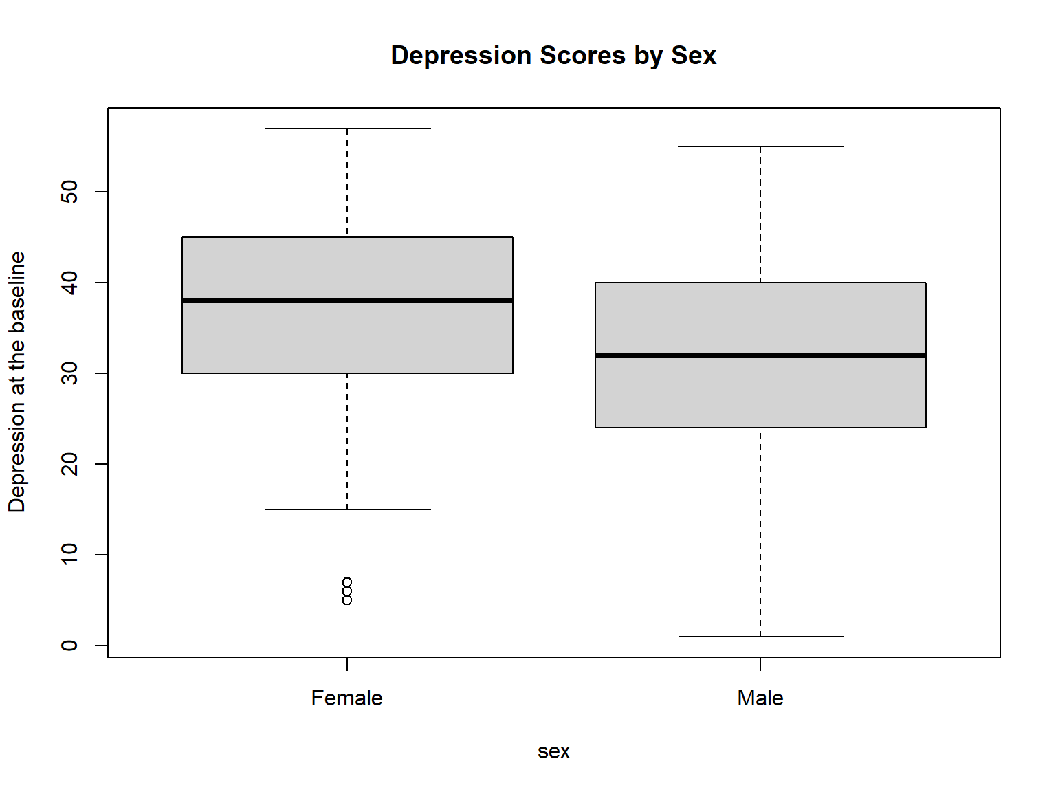
Figure 6.1: Boxplot of depression scores by sex
It seems that female patients have higher levels of depression on average, compared to male patients. Next, we will create two new small datasets (male and female) that consist of only depression scores for each gender group.
male <- subset(medical, sex == "male", select = "depression1")
female <- subset(medical, sex == "female", select = "depression1")
t.test(male, female, conf.level = 0.95, alternative = "two.sided")
    Welch Two Sample t-test

data:  male and female
t = -2.5, df = 87, p-value = 0.02
alternative hypothesis: true difference in means is not equal to 0
95 percent confidence interval:
 -8.418 -0.928
sample estimates:
mean of x mean of y
    31.50     36.18
We can again use the lsr package to get a better output. independentSamplesTTest function does not require us to separate the dataset for each group. We only need to specify the group variable, which is sex in our example. The only thing we need to make sure that the group variable is a factor.
medical$sex <- as.factor(medical$sex)

independentSamplesTTest(formula = depression1 ~ sex,
                        conf.level = 0.95,
                        one.sided = FALSE,
                        data = medical)
   Welch's independent samples t-test

Outcome variable:   depression1
Grouping variable:  sex

Descriptive statistics:
            female   male
   mean     36.175 31.503
   std dev. 12.675 11.758

Hypotheses:
   null:        population means equal for both groups
   alternative: different population means in each group

Test results:
   t-statistic:  2.48
   degrees of freedom:  87.09
   p-value:  0.015

Other information:
   two-sided 95% confidence interval:  [0.928, 8.418]
   estimated effect size (Cohen's d):  0.382
Conclusion: With the significance level of \(\alpha=.05\), we reject the null hypothesis that the average depression score for male and female patients is the same in the population, \(t(87)=-2.5\), \(p < .05\), \(CI_{95}=[-8.42, -0.93]\).
6.5 \(t\)-test with Paired Data
Suppose we have paired data, \(X_1\) and \(X_2\) with \(D=X_1-X_2 \sim N(\mu_D, \sigma)\). We wish to determine whether the two population means (or a single population across two time points), \(\mu_{X_1}\) and \(\mu_{X_2}\), are the same (i.e., \(\mu_D = 0\)) or different (i.e., \(\mu_D \neq 0\)). We test the null hypothesis \(H_0: \mu_X = \mu_Y\) against some alternative hypothesis, with \(\alpha\) level of significance. The test statistic will be:
\[t = \frac{\bar{D}}{\frac{S_D}{\sqrt{n}}}\]
with \(df = n -1\) degrees of freedom. In the formula:
- \(D\) is the difference between two populations (or two time points)
- \(S_D\) is the sample standard deviation of the difference
- \(n\) is the sample size of the second group
If \(t > t_{critical}\) at the \(\alpha\) level of significance, we reject the null hypothesis; otherwise we retain the null hypothesis.
6.5.1 Example
Using the medical dataset, this time we want to know whether patients’ depression scores at the baseline (depression1) are the same as their depression scores after 6 months (depression2). First, let’s see the means for the two variables.
mean(medical$depression1)[1] 32.59mean(medical$depression2)[1] 22.72It seems that the scores at month 6 are much lower. Let’s see if the difference is statistically significant.
t.test(medical$depression1, medical$depression2,
       paired = TRUE, alternative = "two.sided",
       conf.level = 0.95)
    Paired t-test

data:  medical$depression1 and medical$depression2
t = 11, df = 245, p-value <2e-16
alternative hypothesis: true difference in means is not equal to 0
95 percent confidence interval:
  8.021 11.719
sample estimates:
mean of the differences
                   9.87
Let’s repeat the same analysis with the lsr package.
pairedSamplesTTest(formula = ~ depression1 + depression2,
                   conf.level = 0.95,
                   one.sided = FALSE,
                   data = medical)
   Paired samples t-test

Variables:  depression1 , depression2

Descriptive statistics:
            depression1 depression2 difference
   mean          32.585      22.715      9.870
   std dev.      12.112      14.287     14.727

Hypotheses:
   null:        population means equal for both measurements
   alternative: different population means for each measurement

Test results:
   t-statistic:  10.51
   degrees of freedom:  245
   p-value:  <.001

Other information:
   two-sided 95% confidence interval:  [8.021, 11.719]
   estimated effect size (Cohen's d):  0.67
Conclusion: With the significance level of \(\alpha=.05\), we reject the null hypothesis that the average depression scores for the baseline and 6th month are the same in the population, \(t(245)=10.51\), \(p < .001\), \(CI_{95}=[8.02, 11.72]\).
6.6 Analysis of Variance (ANOVA)
Independent-samples \(t\)-test that we have seen earlier is suitable for comparing the means of two independent groups. But, what if there are more than two groups to compare? One could suggest that we run multiple \(t\)-tests to compare all possible pairs and make a decision at the end. However, each statistical test that we run involves a certain level of error (known as Type I error) that leads to incorrect conclusions on the results. Repeating several \(t\)-tests to compare the groups would increase the likelihood of making incorrect conclusions. Therefore, when there are three or more groups to be compared, we follow a procedure called Analysis of Variance – or shortly ANOVA.
Suppose we have \(K\) number of populations. Collect a random sample of size \(n_1\) from population 1, \(n_2\) from population 2, …, \(n_K\) from population \(k\). We assume all populations have the same standard deviation (and they are normally distributed). We wish to test the following null hypothesis:
\[H_0: \mu_1=\mu_2=\mu_3=\dots=\mu_K\] against
\[H_1: H_0 \text{ is false}\]
which means that all of the groups would have equal means in their populations. If at least one of the groups has a significantly different mean, then we would reject the null hypothesis and run post-hoc tests to find out which group(s) are different.
Let \(N = \sum_{k = 1}^{K} n_k\) be the grand total, \((\overline{x}_k = \frac{1}{n_k} \sum_{i = 1}^{n_k} x_{ki}\)) be the sample mean for sample \(k\), and \(\overline{x}_{\cdot} = \frac{1}{N} \sum_{k = 1}^{K} \sum_{i = 1}^{n_k} x_{ki}\) be the grand mean. Then, the \(F\)-statistic is
\[F = \frac{\sum_{k = 1}^{K}\left(\overline{x}_k - \overline{x}_{\cdot}\right)^2/(K - 1)}{\sum_{k = 1}^{K} \sum_{i = 1}^{n_k} \left(x_{ki} - \overline{x}_k\right)^2/(N - K)}\]
with degrees of freedom of \(df_1 = K - 1\) and \(df_2 = N - K\).
If \(F > F_{critical}\) at the \(\alpha\) level of significance, we reject the null hypothesis; otherwise we retain the null hypothesis.
6.6.1 Example
Using the medical dataset, we want to investigate whether patients with different types of substance addition had the same level of depression at the baseline. We will use depression1 and substance for this analysis. Before we begin the analysis, let’s visualize the distribution of depression1 by substance to get a sense of potential group differences.
boxplot(formula = depression1 ~ substance,
        data = medical,
        main = "Depression Scores by Substance Type",
        ylab = "Depression at the baseline")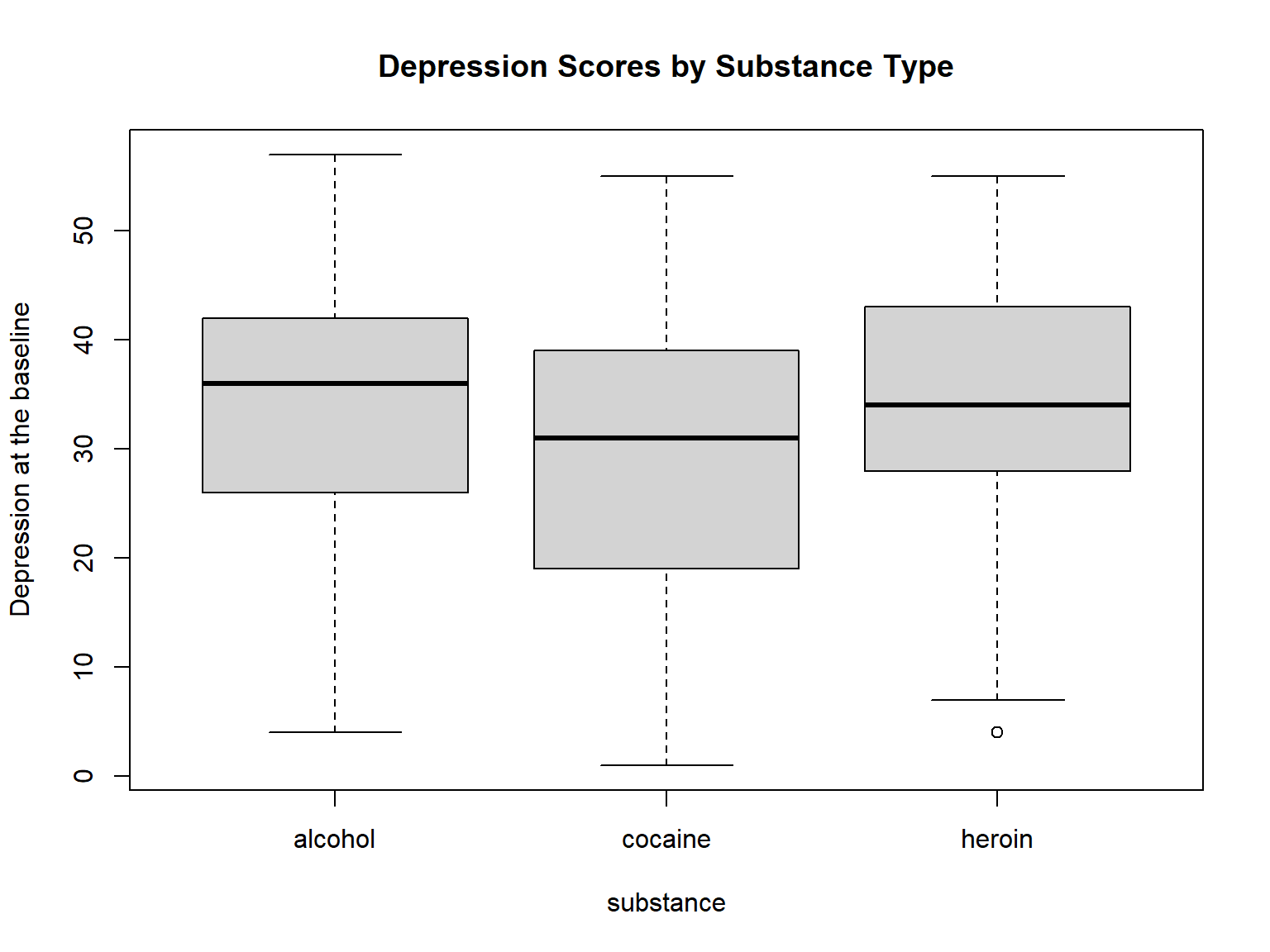
Figure 6.2: Boxplot of depression scores by substance type
The boxplot shows that the means are close across the three groups but we cannot tell for sure if the differences are negligible to ignore. We will use the aov function – which is part of base R.
# Compute the analysis of variance
aov_model1 <- aov(depression1 ~ substance, data = medical)

# Summary of the analysis
summary(aov_model1)
Df Sum Sq Mean Sq F value Pr(>F)
substance 2 1209 605 4.23 0.016 *
Residuals 243 34733 143
---
Signif. codes: 0 '***' 0.001 '**' 0.01 '*' 0.05 '.' 0.1 ' ' 1Conclusion: With the significance level of \(\alpha=.05\), the output shows that \(F(2, 243) = 4.23, p < .05\), indicating that the test is statistically significant and thus we need to reject the null hypothesis of equal group means. This finding also suggests that at least one of the groups is different from the others.
As the ANOVA test is significant, now we can compute Tukey HSD (Tukey Honest Significant Differences) for performing multiple pairwise-comparison between the means of groups. The function TukeyHD() takes the fitted ANOVA as an argument and gives us the pairwise-comparison results.
TukeyHSD(aov_model1) Tukey multiple comparisons of means
95% family-wise confidence level
Fit: aov(formula = depression1 ~ substance, data = medical)
$substance
diff lwr upr p adj
cocaine-alcohol -4.62684 -8.7730 -0.4807 0.0245
heroin-alcohol -0.08964 -4.7249 4.5456 0.9989
heroin-cocaine 4.53720 -0.1281 9.2025 0.0586In the output above,
- diff: difference between means of the two groups
- lwr, upr: the lower and the upper end point of the confidence interval at 95%
- p adj: p-value after adjustment for the multiple comparisons
It can be seen from the output that only the difference between cocaine and alcohol is significant with an adjusted p-value of 0.0245.
We can add other variables into the ANOVA model and continue testing. Let’s include sex as a second variable.
# Substance + Sex
aov_model2 <- aov(depression1 ~ substance + sex, data = medical)
summary(aov_model2)
Df Sum Sq Mean Sq F value Pr(>F)
substance 2 1209 605 4.36 0.0138 *
sex 1 1199 1199 8.65 0.0036 **
Residuals 242 33534 139
---
Signif. codes: 0 '***' 0.001 '**' 0.01 '*' 0.05 '.' 0.1 ' ' 1# Substance + Sex + Substance x Sex
aov_model3 <- aov(depression1 ~ substance*sex, data = medical)
summary(aov_model3) Df Sum Sq Mean Sq F value Pr(>F)
substance 2 1209 605 4.38 0.0135 *
sex 1 1199 1199 8.69 0.0035 **
substance:sex 2 435 218 1.58 0.2083
Residuals 240 33098 138
---
Signif. codes: 0 '***' 0.001 '**' 0.01 '*' 0.05 '.' 0.1 ' ' 1The output shows that sex is also statistically significant in the model; but the interaction of sex and substance is not statisticall significant.
6.7 Exercise 9
Now you will run two hypothesis tests using the variables in the medical dataset:
Run an independent-samples \(t\)-test where you will investigate whether the average depression scores at the baseline (i.e.,
depression1) are the same for suicidal patients (i.e.,suicidal == "yes") and non-suicidal patients (i.e.,suicidal == "no").You will conduct an ANOVA to investigate whether the patients’ physical scores at the baseline (i.e.,
physical1) differ depending on their race (i.e.,race).
6.8 Additional Packages to Consider
There are also additional R packages that might be useful when conducting \(t\)-tests. One of these packages is report (https://github.com/easystats/report). This package automatically produces reports of models and data frames according to best practices guidelines (e.g., APA’s style), ensuring standardization and quality in results reporting.
# Install the activate the package
install.packages("report")
library("report")

# Run an independent-samples t test and create a report
report(t.test(male, female, conf.level = 0.95, alternative = "two.sided"))

# Run ANOVA and create a report
report(aov(depression1 ~ substance + sex, data = medical))
Effect sizes were labelled following Cohen's (1988) recommendations.
The Welch Two Sample t-test testing the difference between male and female (mean of x = 31.50, mean of y = 36.18) suggests that the effect is negative, significant and medium (difference = -4.67, 95% CI [-8.42, -0.93], t(87.09) = -2.48, p < .05; Cohen's d = -0.53, 95% CI [-0.96, -0.10])The ANOVA (formula: depression1 ~ substance + sex) suggests that:
- The main effect of substance is significant and small (F(2, 242) = 4.36, p = 0.014; Eta2 (partial) = 0.03, 90% CI [4.06e-03, 0.08])
- The main effect of sex is significant and small (F(1, 242) = 8.65, p = 0.004; Eta2 (partial) = 0.03, 90% CI [6.71e-03, 0.08])
Effect sizes were labelled following Field's (2013) recommendations.Finally, report also includes some functions to help you write the data analysis paragraph about the tools used.
report(sessionInfo())Analyses were conducted using the R Statistical language (version 4.0.4; R Core Team, 2021) on Windows 10 x64 (build 19043), using the packages skimr (version 2.1.2; Elin Waring et al., 2020), ggplot2 (version 3.3.3; Wickham. ggplot2: Elegant Graphics for Data Analysis. Springer-Verlag New York, 2016.), dplyr (version 1.0.5; Hadley Wickham et al., 2021), kableExtra (version 1.3.4; Hao Zhu, 2021), car (version 3.0.10; John Fox and Sanford Weisberg, 2019), carData (version 3.0.3; John Fox, Sanford Weisberg and Brad Price, 2019), report (version 0.2.0; Makowski et al., 2020) and lsr (version 0.5; Navarro, 2015).
References
----------
- Elin Waring, Michael Quinn, Amelia McNamara, Eduardo Arino de la Rubia, Hao Zhu and Shannon Ellis (2020). skimr: Compact and Flexible Summaries of Data. R package version 2.1.2. https://CRAN.R-project.org/package=skimr
- H. Wickham. ggplot2: Elegant Graphics for Data Analysis. Springer-Verlag New York, 2016.
- Hadley Wickham, Romain François, Lionel Henry and Kirill Müller (2021). dplyr: A Grammar of Data Manipulation. R package version 1.0.5. https://CRAN.R-project.org/package=dplyr
- Hao Zhu (2021). kableExtra: Construct Complex Table with 'kable' and Pipe Syntax. R package version 1.3.4. https://CRAN.R-project.org/package=kableExtra
- John Fox and Sanford Weisberg (2019). An {R} Companion to Applied Regression, Third Edition. Thousand Oaks CA: Sage. URL: https://socialsciences.mcmaster.ca/jfox/Books/Companion/
- John Fox, Sanford Weisberg and Brad Price (2019). carData: Companion to Applied Regression Data Sets. R package version 3.0-3. https://CRAN.R-project.org/package=carData
- Makowski, D., Ben-Shachar, M.S., Patil, I. & Lüdecke, D. (2020). Automated reporting as a practical tool to improve reproducibility and methodological best practices adoption. CRAN. Available from https://github.com/easystats/report. doi: .
- Navarro, D. J. (2015) Learning statistics with R: A tutorial for psychology students and other beginners. (Version 0.5) University of Adelaide. Adelaide, Australia
- R Core Team (2021). R: A language and environment for statistical computing. R Foundation for Statistical Computing, Vienna, Austria. URL https://www.R-project.org/.