7 Correlation and Regression
7.1 Correlation
Correlation measures the degree to which two variables are related to or associated with each other. It provides information on the strength and direction of relationships. The most widely used correlation index, also known as Pearson correlation, is
\[\text{For populations: } \rho = \frac{\sigma_{xy}}{\sigma_x \sigma_y}\]
\[\text{For samples: } r = \frac{S_{xy}}{S_x S_y}\]
Here are some notes on how to interpret correlations:
Correlation can range from -1 to +1.
The sign (either - or +) shows the direction of the correlation
The value of correlation shows the magnitude of the correlation.
As correlations get closer to either -1 or +1, the strength increases.
Correlations near zero indicate very weak to no correlation.
There are many guidelines for categorizing weak, moderate, and strong correlations. Typically, researchers refers to Cohen’s guidelines2 as shown below:
| Correlation | Interpretation |
|---|---|
| 0.1 | Small |
| 0.3 | Moderate |
| 0.5 | Strong |
In R, the cor() function provides correlation coefficients and matrices. For the correlation between two variables (depression1 and mental1):
cor(medical$depression1, medical$mental1)[1] -0.6629For the correlation between multiple variables:
cor(medical[, c("depression1", "mental1", "physical1")]) depression1 mental1 physical1
depression1 1.0000 -0.66289 -0.32000
mental1 -0.6629 1.00000 0.05698
physical1 -0.3200 0.05698 1.00000If some of the variables include missing values, then we can add either use = "complete.obs" (listwise deletion of missing cases) or use = "pairwise.complete.obs" (pairwise deletion of missing cases) inside the cor function.
To test the significance of the correlation, we can use the correlate function from the lsr package:
# Activate the package
library("lsr")

correlate(medical[, c("depression1", "mental1", "physical1")],
          test = TRUE, corr.method="pearson")
CORRELATIONS
============
- correlation type:  pearson
- correlations shown only when both variables are numeric

            depression1    mental1    physical1
depression1           .     -0.663***    -0.320***
mental1          -0.663***       .        0.057
physical1        -0.320***   0.057            .

---
Signif. codes: . = p < .1, * = p<.05, ** = p<.01, *** = p<.001


p-VALUES
========
- total number of tests run:  3
- correction for multiple testing:  holm

            depression1 mental1 physical1
depression1           .   0.000     0.000
mental1           0.000       .     0.373
physical1         0.000   0.373         .


SAMPLE SIZES
============

            depression1 mental1 physical1
depression1         246     246       246
mental1             246     246       246
physical1           246     246       246
In addition to printing correlation matrices, R also provides nice ways to visualize correlations. In the following example, we will use the corrplot function from the corrplot package (Wei and Simko 2017) to draw a correlation matrix plot3.
# Install and activate the package
install.packages("corrplot")
library("corrplot")
# First, we need to save the correlation matrix
cor_scores <- cor(medical[, c("depression1", "mental1", "physical1",
"depression2", "mental2", "physical2")])
# Plot 1 with circles
corrplot(cor_scores, method="circle")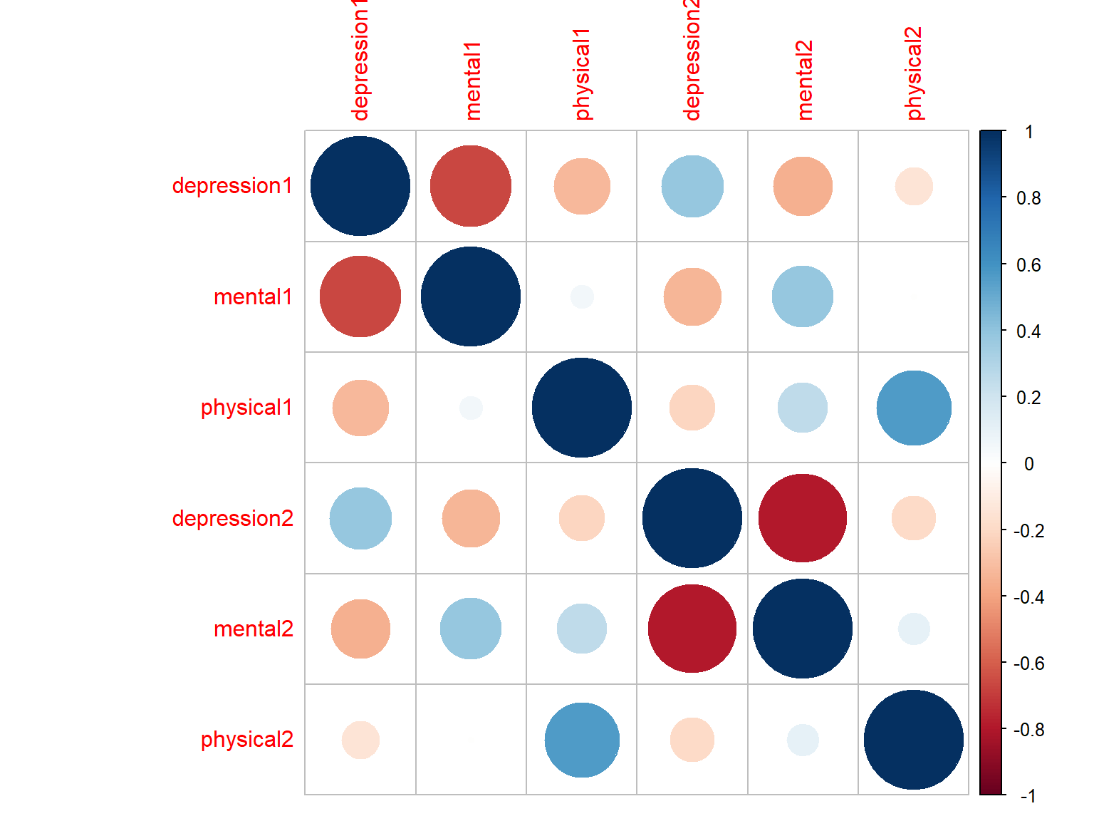
Figure 7.1: Correlation matrix plot with circles
# Plot 2 with colors
corrplot(cor_scores, method="color")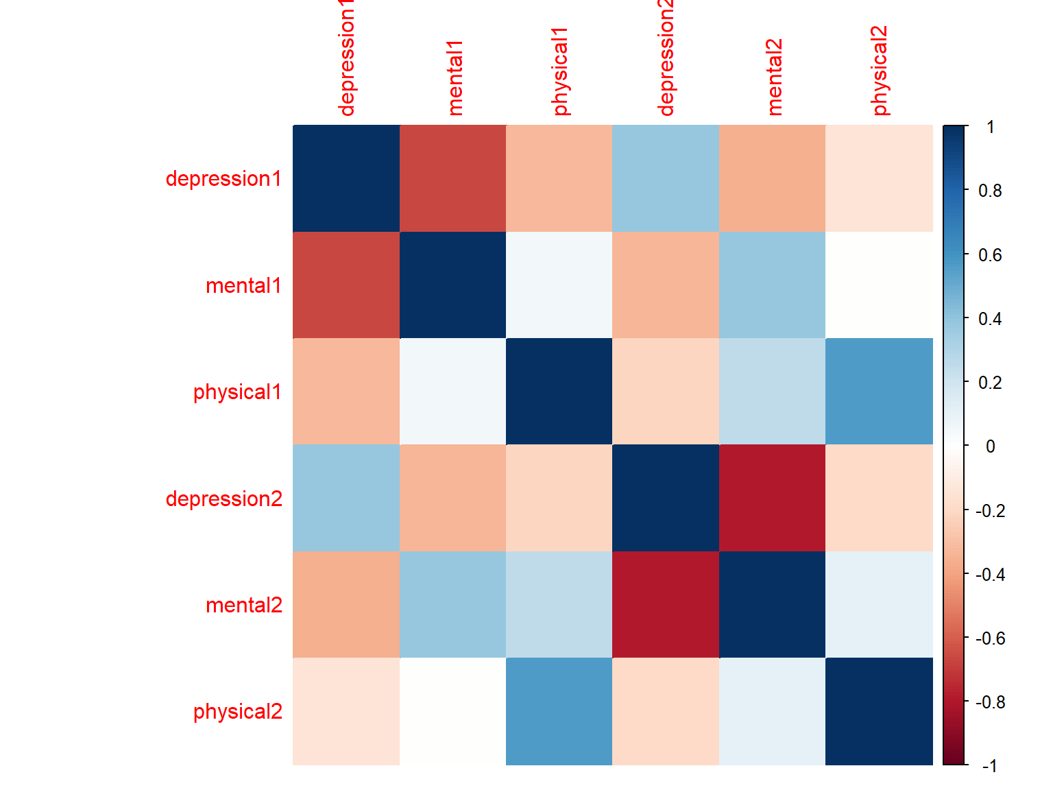
Figure 7.2: Correlation matrix plot with colours
# Plot 3 with numbers
corrplot(cor_scores, method="number")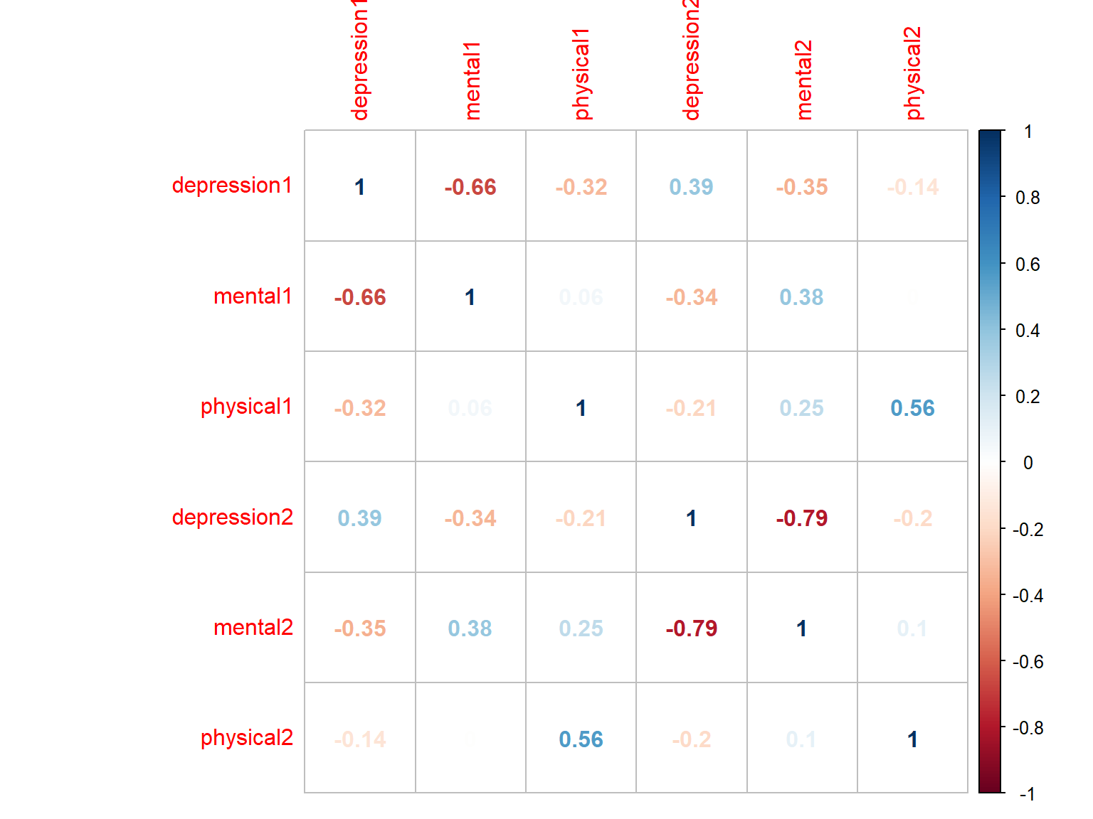
Figure 7.3: Correlation matrix plot with numbers
# Plot 4 with circles + lower triangular
corrplot(cor_scores, method="circle", type="lower")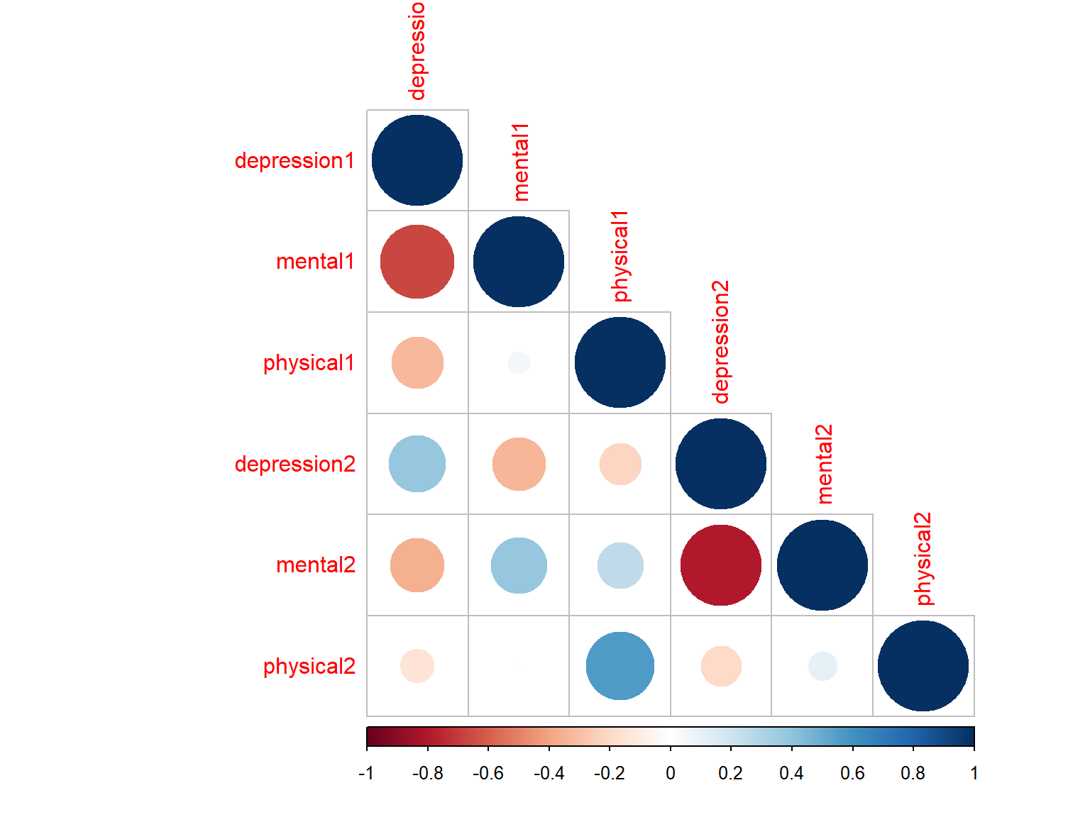
Figure 7.4: Correlation matrix plot with circle and lower triangle
# Plot 5 with circles + lower triangular + ordered correlations
corrplot(cor_scores, method="circle", type="lower", order="hclust")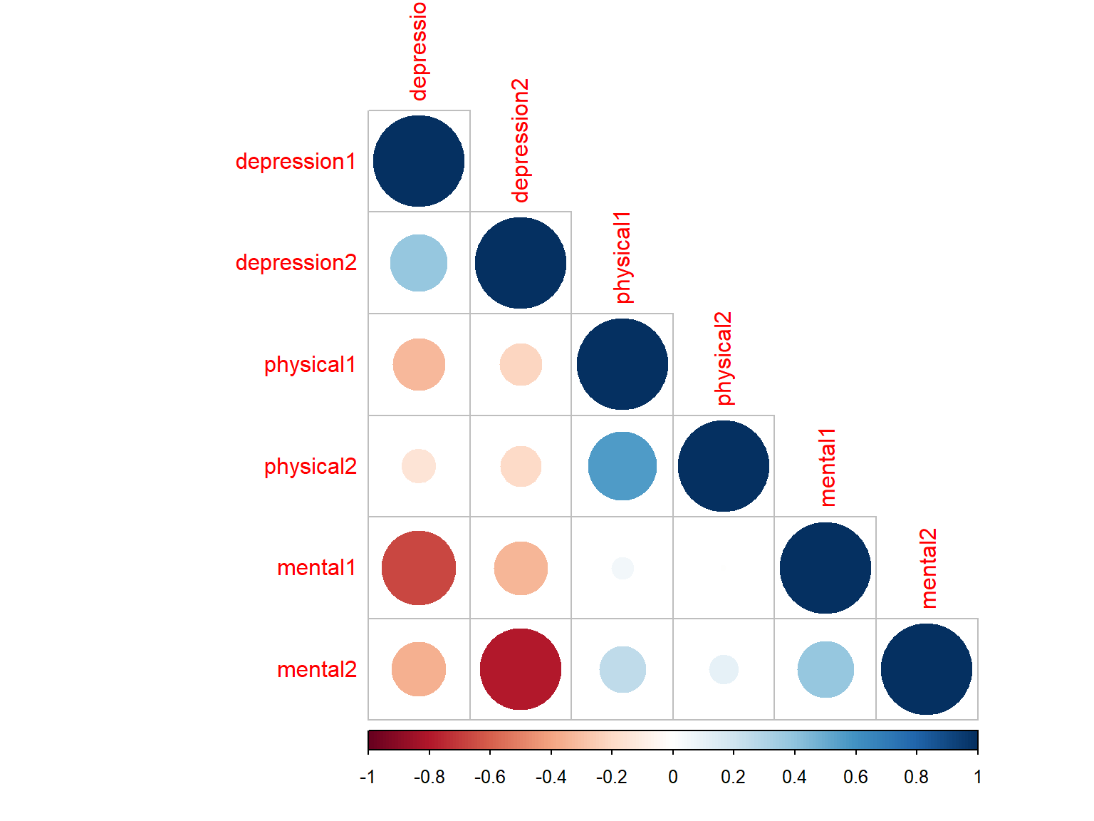
Figure 7.5: Correlation matrix plot with ordered correlations
7.2 Simple Linear Regression
Linear regression is a standard tool that researchers often rely on when analyzing the relationship between some predictors (i.e., independent variables) and an outcome (i.e., dependent variable). In a simple linear regression model, we aim to fit the best linear line to the data based on a single predictor so that the sum of residuals is the smallest. This method is known as “ordinaly least squares” (OLS). Once the regression equation is computed, we can use it to make predictions for a new sample of observations.
If \(Y\) is the dependent variable (DV) and \(X\) is the independent variable (IV), then the formula that describes our simple regression model becomes:
\[Y_i = b_1 X_i + b_0 + \epsilon_i\]
where \(b_1\) is the slope (the increase in \(Y\) for every one unit increase in \(X\)), \(b_0\) is the intercept (the value of \(Y\) when \(X=0\)), and \(\epsilon_i\) is the residual (the difference between the predicted values based on the regression model and the actual values of the dependent variable).
In R, there are many ways to run regression analyses. However, the simplest way to run a regression model in R is to use the lm() function that fits a linear model to a given dataset (see ?lm in the console for the help page). Here are the typical elements of lm():
formula: A formula that specifies the regression model. This formula is of the form DV ~ IV.data: The data frame containing the variables.
7.2.1 Example
Now let’s see how regression works in R. We want to predict patients’ mental scores at the baseline (i.e., mental1) using their depression scores at the baseline (i.e., depression1). To see how this relationship looks like, we can first take a look at the scatterplot as well as the correlation between the two variables.
cor(medical$depression1, medical$mental1)[1] -0.6629\(r = -.66\) is indicating that there is a negative and moderate relationship between the two variables. Although we know that correlation does NOT mean causation, our knowledge or theory from the literature may suggest that these two variables are indeed associated with each other. So, we can move to the next step and plot these two variables in a scatterplot using the `ggplot2 package (see http://sape.inf.usi.ch/quick-reference/ggplot2/colour for many colour options in ggplot2).
# Activate the ggplot2 first
library("ggplot2")

ggplot(data = medical,
       mapping = aes(x = depression1, y = mental1)) +
  geom_point(size = 2, color = "grey25") +
  geom_smooth(method = lm, color = "blue", se = TRUE) +
  labs(x = "Depression scores",
       y = "Mental scores",
       title = "Scatterplot of depression and mental scores at the baseline") +
  theme_bw()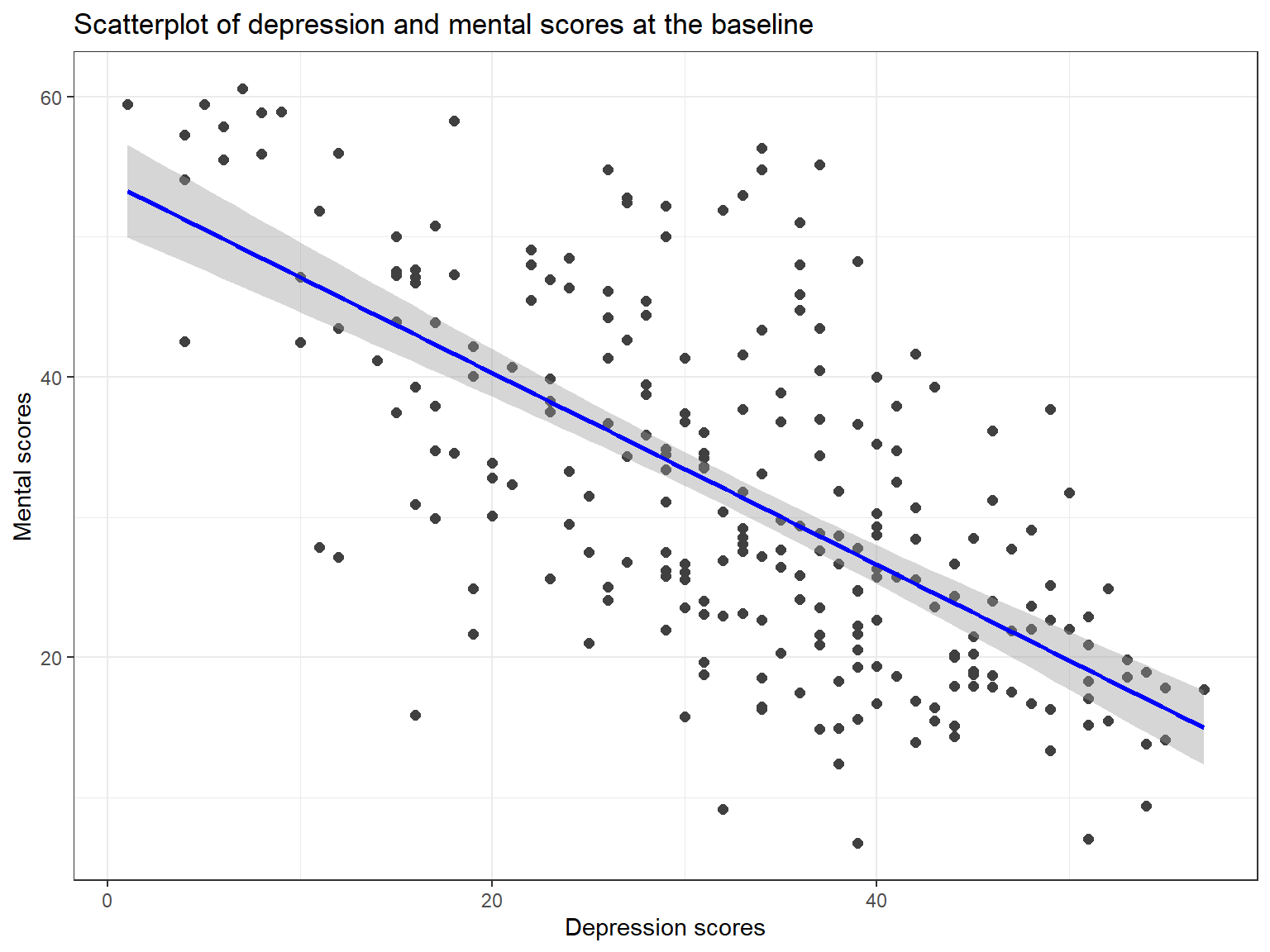
Figure 7.6: Scatterplot of depression and mental scores at the baseline
The scatterplot also confirms that there is a negative relationship between the two variables. Now we can fit a regression model to the data to quantify this relationship.
# Set up the model and save it as model1
model1 <- lm(mental1 ~ depression1, data = medical)

# Print basic model output
print(model1)
Call:
lm(formula = mental1 ~ depression1, data = medical)

Coefficients:
(Intercept)  depression1
     53.948       -0.683
# Print detailed summary of the model
summary(model1)
Call:
lm(formula = mental1 ~ depression1, data = medical)

Residuals:
    Min      1Q  Median      3Q     Max
-27.152  -6.993   0.039   5.853  26.464

Coefficients:
            Estimate Std. Error t value Pr(>|t|)
(Intercept)  53.9477     1.7173    31.4   <2e-16 ***
depression1  -0.6834     0.0494   -13.8   <2e-16 ***
---
Signif. codes:  0 '***' 0.001 '**' 0.01 '*' 0.05 '.' 0.1 ' ' 1

Residual standard error: 9.37 on 244 degrees of freedom
Multiple R-squared:  0.439, Adjusted R-squared:  0.437
F-statistic:  191 on 1 and 244 DF,  p-value: <2e-16
The output shows that our regression equation is:
\[\hat{mental1} = 53.9477 - 0.6834(depression1)\] suggesting that one unit increase in the depression scores corresponds to -0.6834 points increase in the mental scores at the baseline.
t value in the output indicates the individual \(t\) tests for testing whether intercept and slope are significantly different from zero; i.e., \(H_0 = b_0 = 0\) and \(H_0 = b_1 = 0\). The test for the intercept is not really interesting as we rarely care about whether or not the intercept is zero. However, for the slope, we want this test to be significant in order to conclude that the predictor is indeed useful for predicting the dependent variable. In our example, \(t = -13.8\) for the slope and its p-value is less than .001. This indicates that the slope was significantly different from zero (i.e., an important predictor in our model). In the output *** shows the level of significance.
Another important information is \(R^2\), which indicates the proportion of the variance explained by the predictor (depression1) in the dependent variable (mental1). In our model, \(R^2 = 0.439\) – which means \(43.9%\) of the variance in the mental scores can be explained by the depression scores.
There are many guidelines for categorizing for interpreting R-squared values. Researchers often refers to Cohen’s guidelines as shown below:
| R-squared | Interpretation |
|---|---|
| 0.1 | Small |
| 0.09 | Moderate |
| 0.25 | Large |
Using these guidelines, we can say that our model indicates a large effect between the dependent and independent variables.
Finally, the output has additional information about the overall significance of the regression model: \(F(1, 244) = 191, p < .001\), suggesting that the model is statistically significant. This information may not be useful when we have a simple regression model because we already know that our predictor is significantly predicts the dependent variable. However, this information will be more useful when we look at multiple regression where only some variables might be significant, not all of them.
7.3 Multiple Regression
The simple linear regression model that we have discussed up to this point assumes that there is a single predictor variable that we are interested in. However, in many (perhaps most) research projects, we actually have multiple predictors that we want to examine. Therefore, we can extend the linear regression framework to be able to include multiple predictors – which is called multiple regression.
Multiple regression is conceptually very simple. All we do is to add more predictors into our regression equation. Let’s suppose that we are interested in predicting the mental scores at the baseline (mental1) using both the depression scores at the baseline (depression1), the physical scores at the baseline (physical1), and sex (sex). Our new regression equation should look like this:
\[\hat{mental1} = b_0 + b_1(depression1) + b_2(physical1) + b_3(sex)\]
We would hope that the additional variables we include in the model will make our regression model more precise. In other words, we will be able to better predict the mental scores with the help of these predictors. The caveat is that these two variables should be correlated with the dependent variable (i.e., mental scores) but they should not be highly correlated with each other or the other predictor (i.e., depression scores). If this is the case, adding new variables would not bring additional value to the regression model. Rather, the model would have some redundant variables.
7.3.1 Example
Now let’s see how this will look like in R.
# Add physical1 into the previous model
model2 <- lm(mental1 ~ depression1 + physical1, data = medical)

# Print detailed summary of the model
summary(model2)
Call:
lm(formula = mental1 ~ depression1 + physical1, data = medical)

Residuals:
   Min     1Q Median     3Q    Max
-23.51  -6.30  -0.45   6.11  26.79

Coefficients:
            Estimate Std. Error t value Pr(>|t|)
(Intercept)  64.9234     3.5619   18.23  < 2e-16 ***
depression1  -0.7404     0.0510  -14.52  < 2e-16 ***
physical1    -0.1920     0.0549   -3.49  0.00057 ***
---
Signif. codes:  0 '***' 0.001 '**' 0.01 '*' 0.05 '.' 0.1 ' ' 1

Residual standard error: 9.16 on 243 degrees of freedom
Multiple R-squared:  0.466, Adjusted R-squared:  0.462
F-statistic:  106 on 2 and 243 DF,  p-value: <2e-16
The output shows that our new regression equation is:
\[\hat{mental1} = 64.92 -0.74(depression1) -0.19(physical1)\]
Both predictors negatively predict the mental scores and they are statistically significant in the model. Our R-squared value increased to \(R^2=0.466\), suggesting that \(46.6%\) of the variance can be explained by the two predictors that we have in the model.
By looking at the slopes for each predictor, we cannot tell which predictor plays a more important role in the prediction. Therefore, we need to see the standardized slopes – which are directly comparable based on their magnitudes. We can use the jtools package (Long 2021) to visualize the standardized slopes. To use the jtools package, we have to install both jtools and ggstance.
# Install and activate the packages
install.packages(c("jtools", "ggstance"))
library("jtools")
We will use the plot_summ function from the jtools package to visualize the slopes:
plot_summs(model2, scale = TRUE)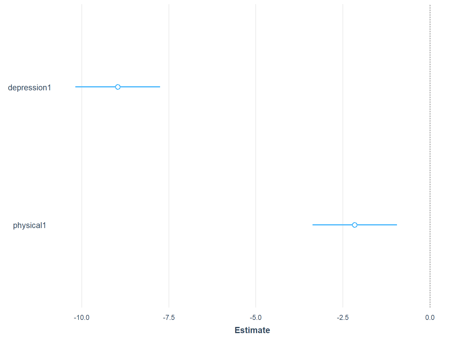
Figure 7.7: Standardized regression coefficients in Model 2
In the plot, the circles in the middle show the location of the standardized slopes (i.e., standardized regression coefficients) for both predictors and the line around the circles represent the confidence interval. We can see from Figure 7.7 that the standardized slope for depression1 is much larger (around -8.5) whereas the standardized slope for physical1 is smaller (around -2). So, we could say that the depression1 is a stronger predictor than physical1 in predicting mental1.
Let’s expand our model by adding sex. Because sex is a categorical variable, R will choose one level of this variable as the reference category and give the results for the other category. The default reference category is selected alphabetically. In the context of sex, the values are male and female. Because f alphabetically comes first, female will be selected as the reference category and we will see the results for male.
# Add sex into the previous model
model3 <- lm(mental1 ~ depression1 + physical1 + sex, data = medical)

# Print detailed summary of the model
summary(model3)
Call:
lm(formula = mental1 ~ depression1 + physical1 + sex, data = medical)

Residuals:
    Min      1Q  Median      3Q     Max
-23.538  -6.409  -0.314   6.040  26.712

Coefficients:
            Estimate Std. Error t value Pr(>|t|)
(Intercept)  64.6403     3.7293   17.33  < 2e-16 ***
depression1  -0.7386     0.0515  -14.33  < 2e-16 ***
physical1    -0.1932     0.0552   -3.50  0.00056 ***
sexmale       0.3689     1.4105    0.26  0.79390
---
Signif. codes:  0 '***' 0.001 '**' 0.01 '*' 0.05 '.' 0.1 ' ' 1

Residual standard error: 9.18 on 242 degrees of freedom
Multiple R-squared:  0.466, Adjusted R-squared:  0.46
F-statistic: 70.5 on 3 and 242 DF,  p-value: <2e-16
The output shows that the estimated slope for sexmale is 0.37; but this slope is not statistically significant as its p-value is 0.79. We could probably conclude that sex does not explain any further variance in the model and therefore we can remove it from the model to keep our regression model simple.
So far we tested three models: Model 1, Model 2, and Model 3. Because the models are nested within each other (i.e., we incrementally added new variables), we can make a model comparison to see if adding those additional predictors brought significant added-value to the models with more predictors. We will use the anova function in base R to accomplish this. This function does not necessarily run the same ANOVA that we discussed earlier. It will compare the models based on their R-squared values.
anova(model1, model2, model3)Analysis of Variance Table
Model 1: mental1 ~ depression1
Model 2: mental1 ~ depression1 + physical1
Model 3: mental1 ~ depression1 + physical1 + sex
Res.Df RSS Df Sum of Sq F Pr(>F)
1 244 21411
2 243 20387 1 1024 12.16 0.00058 ***
3 242 20381 1 6 0.07 0.79390
---
Signif. codes: 0 '***' 0.001 '**' 0.01 '*' 0.05 '.' 0.1 ' ' 1In the output, there are two comparisons:
- Model 1 vs. Model 2
- Model 2 vs. Model 3
The comparison of Model 1 and Model 2 shows that \(F(1,1024)=12.16, p < .001\), suggesting that the larger model (Model 2) explains significantly more variance than the smaller model (Model 1).
The comparison of Model 2 and Model 3 shows that \(F(1,6)=0.07, p=.793\), suggesting that the larger model (Model 3) does NOT explain significantly more variance than the smaller model (Model 2), which confirms our earlier finding that sex did not bring additional value to the model.
We can also compare the three models visually.
plot_summs(model1, model2, model3, scale = TRUE)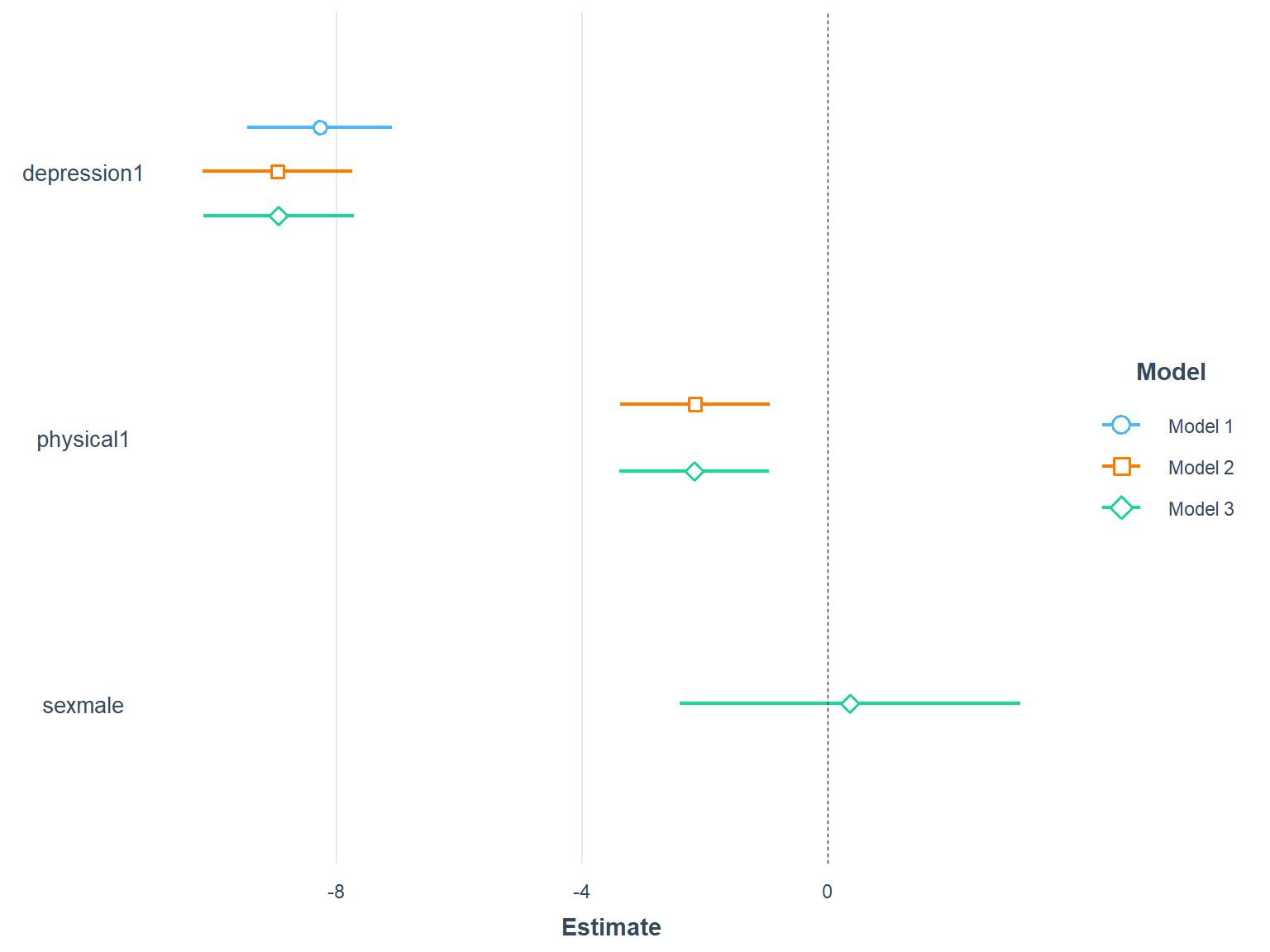
Figure 7.8: Comparison of three models
7.4 Exercise 10
Run a multiple regression model where your dependent variable will be depression2 (i.e., depression scores after 6 months) and your predictors will be:
depression1(i.e., depression scores at the baseline)treat1(i.e., whether the patient received treatment)sex(i.e., patients’ sex)
The questions we can answer are:
- Which variables are significant?
- Do we need all three predictors?
- How is the R-squared value for the model?
7.5 Additional Packages to Consider
There are also additional R packages that might be useful when conducting regression analysis. In the last chapter, we used report (https://github.com/easystats/report) to produce reports of \(t\)-tests. We can use the same package to create reports of regression models.
# Activate the package
library("report")

model <- lm(mental1 ~ depression1 + physical1 + sex, data = medical)

# Print model parameters and additional information
report(model)
We fitted a linear model (estimated using OLS) to predict mental1 with depression1, physical1 and sex (formula: mental1 ~ depression1 + physical1 + sex). The model explains a significant and substantial proportion of variance (R2 = 0.47, F(3, 242) = 70.51, p < .001, adj. R2 = 0.46). The model's intercept, corresponding to depression1 = 0, physical1 = 0 and sex = , is at 64.64 (95% CI [57.29, 71.99], t(242) = 17.33, p < .001). Within this model:
- The effect of depression1 is significantly negative (beta = -0.74, 95% CI [-0.84, -0.64], t(242) = -14.33, p < .001; Std. beta = -0.72, 95% CI [-0.81, -0.62])
- The effect of physical1 is significantly negative (beta = -0.19, 95% CI [-0.30, -0.08], t(242) = -3.50, p < .001; Std. beta = -0.17, 95% CI [-0.27, -0.08])
- The effect of sex [male] is non-significantly positive (beta = 0.37, 95% CI [-2.41, 3.15], t(242) = 0.26, p = 0.794; Std. beta = 0.03, 95% CI [-0.19, 0.25])
Standardized parameters were obtained by fitting the model on a standardized version of the dataset.# Or, print out specific parts of the model output
report_model(model)linear model (estimated using OLS) to predict mental1 with depression1, physical1 and sex (formula: mental1 ~ depression1 + physical1 + sex)report_performance(model)The model explains a significant and substantial proportion of variance (R2 = 0.47, F(3, 242) = 70.51, p < .001, adj. R2 = 0.46)report_statistics(model)beta = 64.64, 95% CI [57.29, 71.99], t(242) = 17.33, p < .001; Std. beta = -0.02, 95% CI [-0.22, 0.17]
beta = -0.74, 95% CI [-0.84, -0.64], t(242) = -14.33, p < .001; Std. beta = -0.72, 95% CI [-0.81, -0.62]
beta = -0.19, 95% CI [-0.30, -0.08], t(242) = -3.50, p < .001; Std. beta = -0.17, 95% CI [-0.27, -0.08]
beta = 0.37, 95% CI [-2.41, 3.15], t(242) = 0.26, p = 0.794; Std. beta = 0.03, 95% CI [-0.19, 0.25]Another useful package for reporting regression results is parameters (https://github.com/easystats/parameters). The goal of this package is to facilitate and streamline the process of reporting results of statistical models, which includes the easy and intuitive calculation of standardized estimates or robust standard errors and p-values.
# Install the activate the package
install.packages("parameters")
library("parameters")

# To view regular model parameters
model_parameters(model)

# To view standardized model parameters
model_parameters(model, standardize = "refit")
Parameter | Coefficient | SE | 95% CI | t(242) | p
-------------------------------------------------------------------
(Intercept) | 64.64 | 3.73 | [57.29, 71.99] | 17.33 | < .001
depression1 | -0.74 | 0.05 | [-0.84, -0.64] | -14.33 | < .001
physical1 | -0.19 | 0.06 | [-0.30, -0.08] | -3.50 | < .001
sex [male] | 0.37 | 1.41 | [-2.41, 3.15] | 0.26 | 0.794 Parameter | Coefficient | SE | 95% CI | t(242) | p
-------------------------------------------------------------------
(Intercept) | -0.02 | 0.10 | [-0.22, 0.17] | -0.23 | 0.818
depression1 | -0.72 | 0.05 | [-0.81, -0.62] | -14.33 | < .001
physical1 | -0.17 | 0.05 | [-0.27, -0.08] | -3.50 | < .001
sex [male] | 0.03 | 0.11 | [-0.19, 0.25] | 0.26 | 0.794 Lastly, performance (https://github.com/easystats/performance) is another useful package for evaluating the quality of model fit for regression models. The package provides several fit indices to evaluate model fit. Also, it has data visualization tools that facilitate model diagnostics.
# Install the activate the package
install.packages("performance")
library("performance")

# Model performance summaries
model_performance(model)

# Check for heteroskedasticity
check_heteroscedasticity(model)

# Comprehensive visualization of model checks
check_model(model)
# Indices of model performance
AIC | BIC | R2 | R2 (adj.) | RMSE | Sigma
-------------------------------------------------------
1794.707 | 1812.234 | 0.466 | 0.460 | 9.102 | 9.177OK: Error variance appears to be homoscedastic (p = 0.346).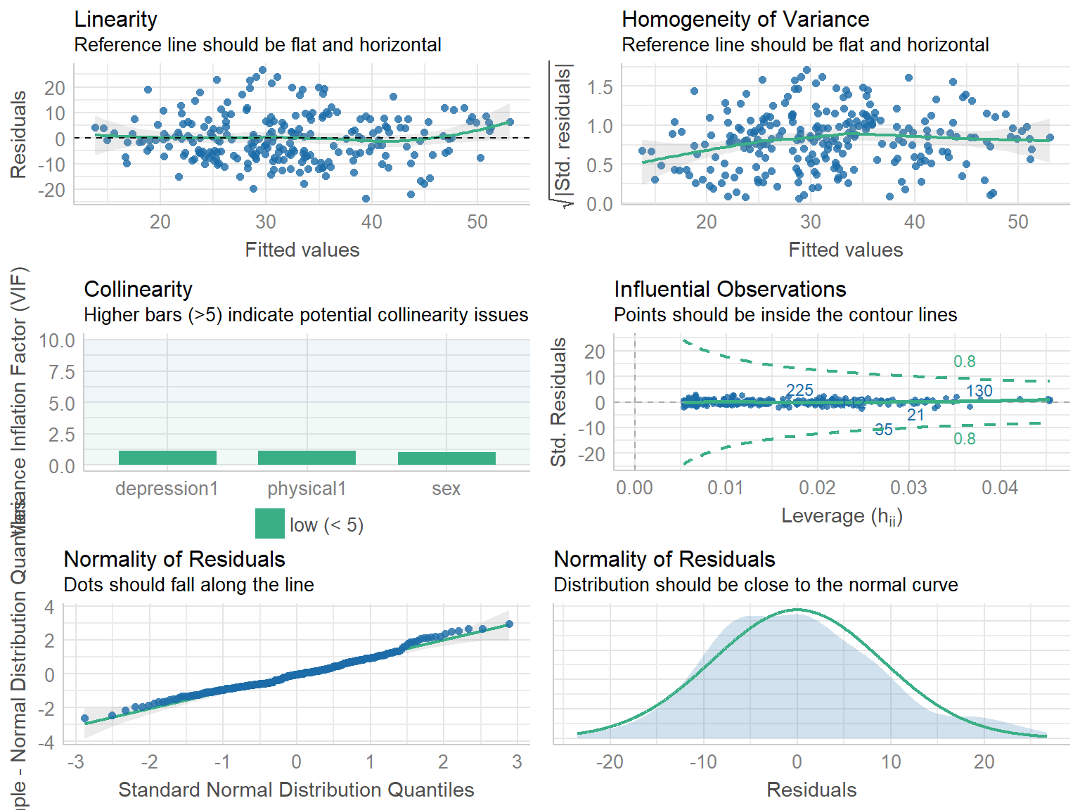
Source: http://imaging.mrc-cbu.cam.ac.uk/statswiki/FAQ/effectSize↩︎
The Gally package also includes a function called
ggcorrto draw correlation matrix plots. Check out this nice tutorial: https://briatte.github.io/ggcorr/ ↩︎